14.1 Zero contours of a bivariate function: roots
The Chebfun2 roots command can compute the zero contours of a function of two variables. For example, here we compute the zero contours of Trott's curve, an example from algebraic geometry [Trott 1997].
cheb.xy;
trott = 144*(x.^4+y.^4) - 225*(x.^2+y.^2) + 350*x.^2.*y.^2 + 81;
r = roots(trott);
plot(r), axis([-1 1 -1 1]), axis square
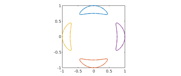
The curves are represented as complex-valued chebfuns (see Section 13.4). For example, here is one of the four components:
r(:,1)
ans =
   chebfun column (1 smooth piece)
       interval       length     endpoint values
[      -1,       1]      576     complex values
vertical scale =   1
Although roots can be outwitted, it is often remarkably accurate. For example, here is the perimeter of a circle of radius 1/2, which we measure by using the fact that the arc length is equal to the 1-norm of the derivative.
f = x.^2 + y.^2 - 1/4;
perimeter = norm(diff(roots(f)),1)
exact_perimeter = pi
perimeter =
   3.141592653589794
exact_perimeter =
   3.141592653589793
For some more exotic examples of zero curves computed by roots, see the 2D Approximation section of the Chebfun examples collection at www.chebfun.org.
14.2 Zeros of a pair of bivariate functions: roots again
Chebfun2 roots can also find zeros of bivariate systems, i.e., solutions to $f(x,y) = g(x,y) = 0$. Generically, these are isolated points.
For example, which points on Trott's curve intersect the circle of radius $0.9$?
g = x.^2 + y.^2 - .9^2;
r = roots(trott,g)
plot(roots(trott),'b'), hold on
plot(roots(g),'r')
MS = 'markersize';
plot(r(:,1),r(:,2),'.k',MS,20)
axis([-1 1 -1 1]), axis square, hold off
r =
  -0.799441089368585  -0.413393208252350
  -0.799441089368583   0.413393208252352
  -0.413393208252347  -0.799441089368586
  -0.413393208252346   0.799441089368587
   0.413393208252345  -0.799441089368587
   0.413393208252344   0.799441089368588
   0.799441089368588  -0.413393208252343
   0.799441089368587   0.413393208252346
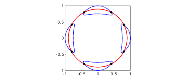
The solutions to bivariate polynomial systems and intersections of curves are typically computed to full machine precision.
14.3 Intersections of curves
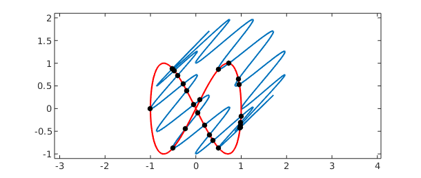
The problem of determining the intersections of real parameterised complex curves can be expressed as a bivariate rootfinding problem. For instance, here are the intersections between the 'splat' curve [Güttel 2010] and a 'figure-of-eight' curve.
t = chebfun('t',[0,2*pi]);
sp = exp(1i*t) + (1+1i)*sin(6*t)^2;      % splat curve
figof8 = cos(t) + 1i*sin(2*t);           % figure of eight curve
plot(sp), hold on
plot(figof8,'r'), axis equal

d = [0 2*pi 0 2*pi];
f = chebfun2(@(s,t) sp(t)-figof8(s),d);  % rootfinding
r = roots(real(f),imag(f));              % calculate intersections
spr = sp(r(:,2));
plot(real(spr),imag(spr),'.k',MS,20), ylim([-1.1 2.1])
hold off
Chebfun2 rootfinding is based on an algorithm described in [Nakatsukasa, Noferini & Townsend 2014].
14.4 Global optimisation: max2, min2, and minandmax2
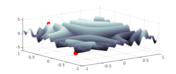
Chebfun2 also provides functionality for global optimisation. Here is an example where we plot the minimum and maximum as red dots.
f = sin(30*x.*y) + sin(10*y.*x.^2) + exp(-x.^2-(y-.8).^2);
[mn mnloc] = min2(f);
[mx mxloc] = max2(f);
plot(f), hold on
plot3(mnloc(1),mnloc(2),mn,'.r',MS,40)
plot3(mxloc(1),mxloc(2),mx,'.r',MS,30)
zlim([-6 6]), colormap('bone'), hold off
If both the global maximum and minimum are required, it is roughly twice as fast to compute them at the same time by using the minandmax2 command. For instance,
tic; [mn mnloc] = min2(f);  [mx mxloc] = max2(f); t = toc;
fprintf('min2 and max2 separately = %5.3fs\n',t)
tic; [Y X] = minandmax2(f); t = toc;
fprintf('minandmax2 command = %5.3fs\n',t)
min2 and max2 separately = 0.306s
minandmax2 command = 0.093s
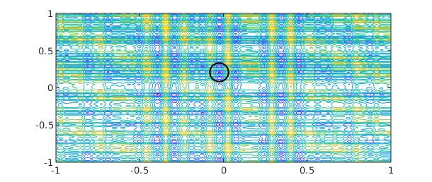
Here is a complicated function from the 2002 SIAM 100-Dollar, 100-Digit Challenge [Bornemann et al. 2004]. Chebfun2 computes its global minimum in a fraction of a second:
tic
f = cheb.gallery2('challenge');
[minval,minpos] = min2(f);
minval
toc
minval =
  -3.306868647474791
Elapsed time is 0.182211 seconds.
The result closely matches the correct solution, computed to 10,000 digits by Bornemann et al.:
exact = -3.306868647475237280076113
exact = -3.306868647475237
Here is a contour plot of this wiggly function, with the minimum circled in black:
colormap('default'), contour(f), hold on
plot(minpos(1),minpos(2),'ok',MS,20), hold off
14.5 Critical points
The critical points of a smooth function of two variables can be located by finding the zeros of $\partial f/ \partial y = \partial f / \partial x = 0$. This is a rootfinding problem. For example,
f = (x.^2-y.^3+1/8).*sin(10*x.*y);
r = roots(gradient(f));                       % critical points
plot(roots(diff(f,1,2)),'b'), hold on         % zero contours of f_x
plot(roots(diff(f)),'r')                      % zero contours of f_y
plot(r(:,1),r(:,2),'k.',MS,24)                % extrema
axis([-1,1,-1,1]), axis square
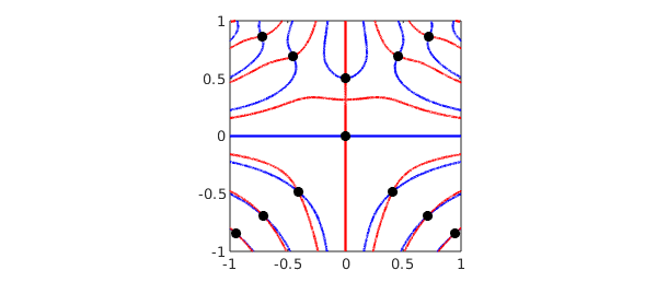
There is a new command here called gradient that computes the gradient vector and represents it as a chebfun2v object. The roots command then solves for the isolated roots of the bivariate polynomial system represented in the chebfun2v representing the gradient. For more information about gradient, see Chapter 15.
14.6 Infinity norm
The $\infty$-norm of a function is the maximum absolute value in its domain. It can be computed by passing the argument inf to the norm command.
f = sin(30*x.*y);
norm(f,inf)
ans =
   1.000000000000003
14.7 References
[Bornemann et al. 2004] F. Bornemann, D. Laurie, S. Wagon and J. Waldvogel, The SIAM 100-Digit Challenge: A Study in High-Accuracy Numerical Computing, SIAM 2004.
[Güttel 2010] S. Güttel, "Area and centroid of a 2D region", http://www.chebfun.org/examples/geom/Area.html.
[Nakatsukasa, Noferini & Townsend 2014] Y. Nakatsukasa, V. Noferini and A. Townsend, "Computing the common zeros of two bivariate functions via Bezout resultants", Numerische Mathematik 129 (2015), 181--209.
[Trott 2007] M. Trott, "Applying GroebnerBasis to three problems in geometry", Mathematica in Education and Research, 6 (1997), 15-28.