In this example we explore the approximation properties of Chebyshev interpolation for entire functions, that is, functions that are analytic everywhere in the complex plane.
1. Analytic functions
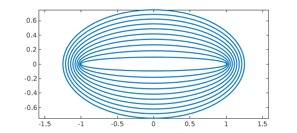
In the following discussion, it will be helpful to utilise the notion of a Bernstein $r$-ellipse, which we define as the image of the circle $|z|=r$ under the mapping $x = (z + z^{-1}) / 2$. Here are some such ellipses, which we denote by $E_r$:
rr = 1 + (1:10)/10;
circ = exp(1i*chebfun('t',[0 2*pi]));
CO = 'color'; blue = [0 .45 .74]; MS = 'markersize';
for k = 1:numel(rr)
    rho = rr(k);
    plot((rho*circ + (rho*circ)^(-1))/2,CO,blue), hold on
end
hold off, axis equal
Suppose we have a function $f$ that is analytic on $[-1,1]$ and that can be analytically continued to the closed $r$-ellipse for some $r > 1$. Then [1, Chap. 8], the $\infty$-norm error arising from interpolating $f$ by a polynomial in $n+1$ Chebyshev points is
$$ \max | f - p_n | \leq \frac{4 M}{r^n (r-1)}, $$
where $M$ is the maximum absolute value taken by $f$ on the ellipse $E_r$. This is a geometric rate of convergence. If we require an accuracy of $0 < \varepsilon < 1$ for our approximations, then it will suffice to obtain the smallest $n$ satisfying
$$ \frac{4 M}{r^n (r-1)} \leq \varepsilon. $$
Some trivial rearrangement of this expression gives
$$ \frac{\log(4/\varepsilon) - \log(r-1) + \log(M)}{\log(r)} \leq n. $$
Choosing an $n$ larger than this will ensure that the interpolant is of accuracy $\varepsilon$.
2. Oscillatory entire functions
When the function $f$ is entire, one may expect the convergence to be even better than geometric, and this is indeed the case. Consider for example, for some positive integer $N$, the entire function
$$ f(x) = \sin(\pi N x). $$
Because $f$ is analytic in the entire complex plane, the convergence result above must hold for any value of $r > 1$. An estimate for the parameter $M$ may be obtained by observing that on a given ellipse, a complex exponential is maximised where the ellipse intersects the (negative) imaginary axis, i.e.,
$$ M \leq \frac{1}{2} \exp(\pi N \frac{r-r^{-1}}{2}). $$
Since this relationship holds for every $r > 1$, we must find the minimum value of the following expression over all $r > 1$,
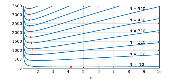
$$ \frac{\log(2/e) - \log(r-1) + \pi N \frac{r-r^{-1}}{2}}{ \log(r) }. $$
For a given oscillation parameter $N$ and precision $\varepsilon$, this may be accomplished using Chebfun. This provides an interesting way to validate the performance of the Chebfun constructor. The plot below shows the function on the LHS of the equation above plotted for different values of $N$. The minimum of each function --- and the estimate for the minimum Chebfun degree required for accuracy $\varepsilon = \varepsilon_{mach}$ --- is plotted in each case as a red dot.
ee = eps; NN = 10:100:1010;
estimates = zeros(numel(NN),1);
chebdegrees = estimates;
for k = 1:numel(NN)
    N = NN(k);
    P = @(p) (log(2/ee) - log(p-1) + N*pi/2*(p-1/p))/log(p);
    PP = chebfun(P,[1.01 10]);
    [mn,pos]= min(PP);
    estimates(k) = mn;
    ff = chebfun(@(x) sin(pi*N*x),'eps',ee);
    chebdegrees(k) = length(ff)-1;
    plot(PP,CO,blue), hold on
    plot(pos,mn,'.r',MS,12)
end
text(8.02,200,  sprintf('N = %3i',NN(1)))
text(8.02,800,  sprintf('N = %3i',NN(2)))
text(8.02,1450, sprintf('N = %3i',NN(3)))
text(8.02,2100, sprintf('N = %3i',NN(4)))
text(8.02,2700, sprintf('N = %3i',NN(5)))
text(8.02,3350, sprintf('N = %3i',NN(6)))
hold off, xlabel('\rho')
shg, grid on, ylim([0 3.5e3])
How do these estimates for the length of the polynomial interpolant compare with Chebfun lengths resulting from Chebfun's adaptive construction process?
est = ceil(estimates);
fprintf('            function        estimate   chebfun length \n')
for k = 1:numel(NN)
    fprintf('         sin( %4i pi x)      %4i          %4i \n',...
                                    NN(k),est(k),chebdegrees(k))
end
fprintf('\n')
            function        estimate   chebfun length
         sin(   10 pi x)        69            67
         sin(  110 pi x)       427           417
         sin(  210 pi x)       761           745
         sin(  310 pi x)      1090          1071
         sin(  410 pi x)      1415          1413
         sin(  510 pi x)      1739          1717
         sin(  610 pi x)      2062          2037
         sin(  710 pi x)      2384          2357
         sin(  810 pi x)      2705          2677
         sin(  910 pi x)      3025          2995
         sin( 1010 pi x)      3346          3315
Very close!
For more, including the definition of the "Chebfun ellipse" of a function, see [1].
References
- L.N. Trefethen, Approximation Theory and Approximation Practice, Extended Edition, SIAM, 2019.