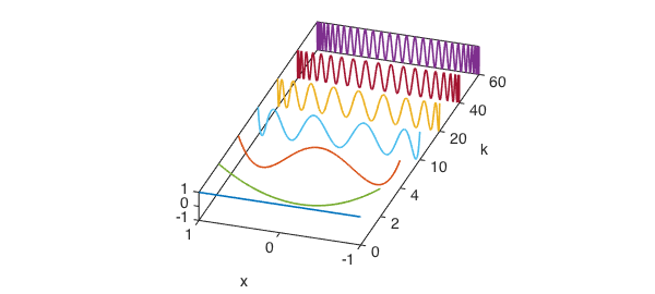
Attractive 3D plots of several Chebyshev polynomails appear in both Fornberg's book [1] (p. 159) and Higham & Higham's book [2] (p. 259). Here are similar plots reproduced in Chebfun.
k = [0 2 4 10 20 40 60];
x = chebfun('x'); one = 1 + 0*x;
FS = 'fontsize'; fs = 14;
for j = 1:length(k)
  plot3(j*one,x,chebpoly(k(j)),'linewidth',1.6), hold on
end
axis([1 length(k) -1 1 -1 1])
box on
set(gca,'dataaspectratio',[1 0.75 4]), view(-72,28)
set(gca,'xticklabel',k)
xlabel('k',FS,fs), ylabel('x',FS,fs), set(gca,FS,fs)
h = get(gca,'xlabel'); set(h,'position',get(h,'position')+[1.5 0.1 0])
h = get(gca,'ylabel'); set(h,'position',get(h,'position')+[0 0.25 0])
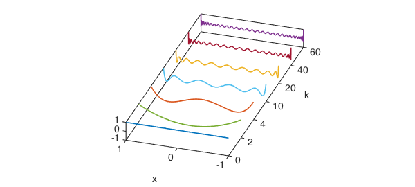
Fornberg also includes the Legendre polynomials for comparison. This can be easily done in Chebfun by replacing chebpoly with legpoly above. Here is the result:
clf;
for j = 1:length(k)
  plot3(j*one,x,legpoly(k(j)),'linewidth',1.6), hold on
end
axis([1 length(k) -1 1 -1 1])
box on
set(gca,'dataaspectratio',[1 0.75 4]), view(-72,28)
set(gca,'xticklabel',k)
xlabel('k',FS,fs), ylabel('x',FS,fs), set(gca,FS,fs)
h = get(gca,'xlabel'); set(h,'position',get(h,'position')+[1.5 0.1 0])
h = get(gca,'ylabel'); set(h,'position',get(h,'position')+[0 0.25 0])
References
-
B. Fornberg, A Practical Guide to Pseudospectral Methods, Cambridge University Press, 1996.
-
D. J. Higham and N. J. Higham, Matlab Guide, 2nd ed., SIAM, 2005.