Conformal mapping of an L-shaped region

The problem of conformally mapping a simply connected domain $\Omega$ to the unit disk, with $f(z_c) = 0$ for a given point $z_c\in \Omega$, can be reduced to a Laplace problem on $\Omega$. If $u$ is a real harmonic function that satisfies $u(z) = -\log|z-z_c|$ on the boundary of $\Omega$, then the conformal map is $f(z) = (z-z_c)\exp (u(z) + i v(z))$, where $v$ is the harmonic conjugate of $u$. To solve this Laplace problem numerically, an easy method is to expand $u$ as a linear combination of a suitable family of harmonic functions -- real and imaginary parts of analytic functions -- and find expansion coefficients by least-squares fitting in a set of sample points on the boundary [2,3].

This process gives the "boundary correspondence function", the homeomorphism between the boundary of $\Omega$ and the unit circle. From here, one can then approximate both $f$ and its inverse by rational functions using AAA approximation as described in [1], invoking the the Chebfun aaa command. The resulting representations of $f$ and $f^{-1}$ can typically be evaluated in microseconds per point.

Here we apply this idea to a simple example of "Schwarz--Christoffel mapping without the Schwarz--Christoffel formula". The following commands determine the map of an L-shaped domain. We make use of an expansion basis consisting of two kinds of terms: powers $(z-z_0)^k$ for a point $z_0$ interior to $\Omega$, and fractional powers $z^{2k/3}$ to handle the singularity at the reentrant corner at $z=0$.

  tic, N = 24;
  format short, warning off                       % suppress Froissart message
  Z = 1i*(1-tanh(12*linspace(1,0,5*N)'));         % sample pts on bndry
  Z = [Z(1:end-1); chebpts(2*N,[1i -1+1i])];
  Z = [Z(1:end-1); chebpts(2*N,[-1+1i -1-1i])];
  a = exp(.25i*pi);                               % 45 degree rotation
  Z = a*[Z/a; conj(Z(end-1:-1:1)/a)];
  mZ = a^3*Z/norm(Z,inf);                         % avoid branch cut
  z0 = -.5-.5i; cZ = (Z-z0)/norm(Z-z0,inf);
  k1 = (0:N); k2 = (1:N);                         % exponents for (z-z0)^k terms
  m1 = k1*(2/3); m2 = k2*(2/3);
  m1(3:3:end) = []; m2(3:3:end) = [];             % exponents for z^(2k/3) terms
  A = [real(cZ.^k1) imag(cZ.^k2) ...              % least-squares matrix
       real(mZ.^m2) imag(mZ.^m2)];
  zc = -.2-.2i;
  U = -log(abs(Z-zc));                            % right-hand side
  c = A\U;                                        % solve the problem
  boundary_err = norm(A*c-U,inf)                  % measure residual
  V = [imag(cZ.^k1) -real(cZ.^k2) ...             % conjugate harmonic fun
       imag(mZ.^m2) -real(mZ.^m2)]*c;
  W = (Z-zc).*exp(U+1i*V); W = W/W(1);            % boundary correspondence
  [f,pol] = aaa(W,Z,'tol',10*boundary_err);       % conformal map
  [finv,polinv] = aaa(Z,W,'tol',10*boundary_err); % inverse map

boundary_err =
   5.1268e-07

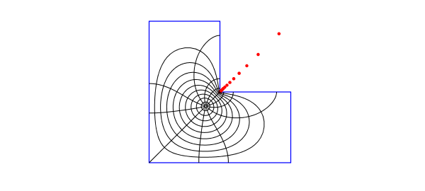
Here is a plot of the map. The red dots show the poles of the AAA approximation, which represents $f$ to about six digits of accuracy. There are also a few more poles off-scale.

  LW = 'linewidth'; MS = 'markersize';
  plot(Z,'b',LW,1)
  axis(1.1*[-1 1 -1 1]), axis square, hold on, axis off
  plot(pol,'.r',MS,10)
  ray = chebpts(100); ray = ray(ray>=0);
  for th = 2*pi*(1:12)/12, plot(finv(exp(1i*th)*ray),'k',LW,.5), end
  circ = exp(2i*pi*(0:200)/200);
  for r = .1:.1:.9, plot(finv(r*circ),'k',LW,.5), end, hold off
  number_of_poles_of_f = length(pol)

number_of_poles_of_f =
    27

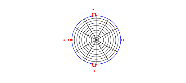
The curves just plotted are the images under $f^{-1}$ of circles and radial lines in the unit disk, which we now plot. The red dots are the poles of $f^{-1}$.

  plot(W,'b',LW,1)
  axis(1.4*[-1 1 -1 1]), axis square, hold on, axis off
  plot(polinv,'.r',MS,10)
  for th = 2*pi*(1:12)/12, plot(exp(1i*th)*ray,'k',LW,.5), end
  for r = .1:.1:.9, plot(r*circ,'k',LW,.5), end, hold off
  number_of_poles_of_finv = length(polinv)

number_of_poles_of_finv =
    44

A well-known effect, going back to Newman and 1964 and Zolotarev in the 19th century, is that poles of rational approximations tend to cluster exponentially near singularities [6]. Let us examine this effect for the first plot above, where the poles cluster near the reentrant corner. Here are the distances of those poles from the singularity plotted on a log scale. The curving down at the left edge is a known phenomenon, whcih is modeled in equation (3.2) of [2] and explained in [6].

distances = sort(abs(pol(real(pol)>0 & imag(pol)>0)));
clf, semilogy(distances,'.-',MS,12,LW,.5), grid on
title('distances of poles to singularity')

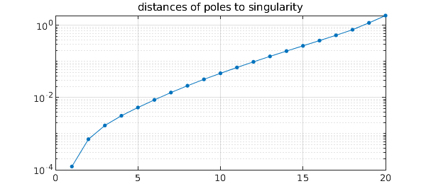
The exponential clustering is striking. The see it quantitatively, we can look at the ratios of successive distances:

ratios = distances(2:end)./distances(1:end-1)

For much more about numerical conformal mapping of regions with corners, see [4] and also the code confmap available at [5].

total_time_for_this_example = toc

total_time_for_this_example =
    1.3084

[1] A. Gopal and L. N. Trefethen, Representation of conformal maps by rational functions, Numer. Math. 142 (2019), 359-382.

[2] A. Gopal and L. N. Trefethen, Solving Laplace problems with corners singularities via rational functions, SIAM J. Numer. Anal. 57 (2019), 2074-2094.

[3] L. N. Trefethen, Conformal mapping in Chebfun, Chebfun example chebfun.org/examples/complex/ConformalMapping.html.

[4] L. N. Trefethen, Numerical conformal mapping with rational functions, Computational Methods and Function Theory, 20 (2020), 369-387.

[5] L. N. Trefethen, confmap.m code, people.maths.ox.ac.uk/trefethen/lightning.html.

[6] L. N. Trefethen, Y. Nakatsukasa, and J. A. C. Weideman, Exponential node clustering at singularities for rational approximation, quadrature, and PDEs, Numerische Mathematik, 147 (2021), 227-254.

Conformal mapping of an L-shaped region

Nick Trefethen, October 2019 in complexdownload·view on GitHub