Field of values and numerical abscissa

If A is a matrix, the field of values F(A) is the nonempty bounded convex set in the complex plane consisting of all the Rayleigh quotients of A, that is, all the numbers q'Aq, where q is a unit vector and q' is its conjugate transpose.

The standard method for computing the field of values numerically is an algorithm due to C. R. Johnson in 1978 based on finding the maximum and minimum eigenvalues of (A+A')/2, then "rotating" this computation around in the complex plane [1]. This algorithm is implemented in the Chebfun command FOV, which is listed at the end of this Example.

Generically the boundary of the field of values is smooth, but it is not always smooth. Chebfun's 'splitting' feature enables FOV to compute this boundary in either situation, smooth or not.

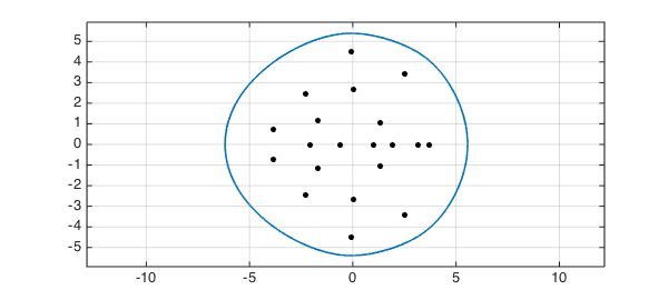
For example, here are the eigenvalues and field of values of a random matrix of dimension 20. This is a case where the boundary is smooth.

rng(1), A = randn(20);
LW = 'linewidth'; lw = 1.6; MS = 'markersize'; ms = 18;
FA = fov(A);
figure, plot(FA,LW,lw), axis equal, grid on
ax = axis; axis(1.1*ax)
hold on, plot(eig(A),'.k',MS,ms)

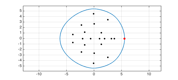
The numerical abscissa of A is the maximum real part of its field of values:

[alpha,maxtheta] = max(real(FA))

alpha =
   5.556701165271451
maxtheta =
     0

Here we add it to the plot as a red dot:

plot(real(FA(maxtheta)),imag(FA(maxtheta)),'.r',MS,24)

You can also find the numerical abscissa without Chebfun:

alpha = max(eig((A+A')/2))

alpha =
   5.556701165271411

Now let's consider a matrix B defined as a diagonal matrix with the same eigenvalues as A. In this case the boundary of the field of values is a polygon:

B = diag(eig(A));
FB = fov(B);
hold off, plot(real(FB),imag(FB),'b',LW,lw,'jumpline',{'b',LW,lw})
hold on, plot(eig(B),'.k',MS,ms), axis(1.1*ax), axis equal, grid on
[alpha,maxtheta] = max(real(FB));
plot(real(FB(maxtheta)),imag(FB(maxtheta)),'.r',MS,24)

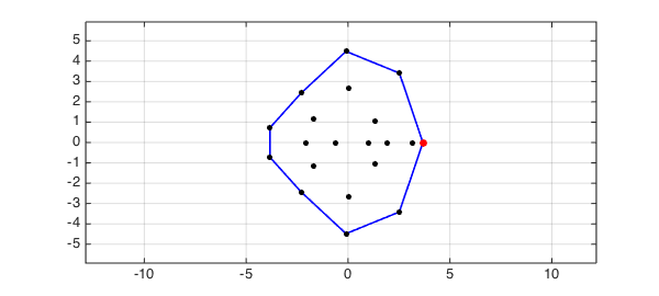
Since the field of values is not smooth, its boundary is a chebfun with several pieces:

FB

FB =
   chebfun column (10 smooth pieces)
       interval       length   endpoint values  
[       0,    0.33]        1       3.7      3.7 
[    0.33,     1.2]        1    complex values 
[     1.2,     2.3]        1    complex values 
[     2.3,     2.4]        1    complex values 
[     2.4,     3.1]        1    complex values 
[     3.1,     3.9]        1    complex values 
[     3.9,       4]        1    complex values 
[       4,     5.1]        1    complex values 
[     5.1,       6]        1    complex values 
[       6,     6.3]        1       3.7      3.7 
Epslevel = 1.110223e-15.  Vscale = 4.481235e+00.  Total length = 10.

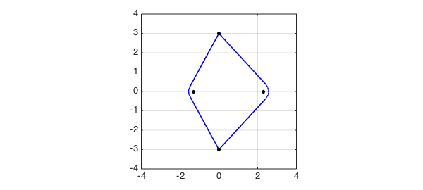
Finally, here's an example where the boundary of the field of values mixes smooth curves with straight segments:

C = [0 3 0 0; -3 0 0 0; 0 0 0 3; 0 0 1 1]
FC = fov(C);
hold off, plot(real(FC),imag(FC),'b',LW,lw,'jumpline',{'b',LW,lw})
axis(4*[-1 1 -1 1]), axis square, grid on
hold on, plot(eig(C),'.k',MS,ms)

C =
     0     3     0     0
    -3     0     0     0
     0     0     0     3
     0     0     1     1

Here is a listing of FOV. Note that the numerical computations are carried out in just about 10 lines of code.

type fov

function [f, lineSegs, theta] = fov(A, pref)
%FOV   Field of values (numerical range) of matrix A.
%   F = FOV(A), where A is a square matrix, returns a CHEBFUN F with domain [0
%   2*pi]. The image F([0 pi]) is a curve describing the extreme points of the
%   boundary of the field of values A, a convex region in the complex plane. 
%
%   For a generic matrix, the boundary of the field of values is smooth and all
%   boundary points are extreme points. If A is normal, the field of values is
%   the convex hull of the eigenvalues of A, so the extreme points consist only
%   of the eigenvalues and hence F has one constant piece for each eigenvalue,
%   so it is not continuous on [0, 2*pi].
%  
%   The numerical abscissa of A is equal to max(real(F)), though this is much
%   better computed as max(real(eig(A + A')))/2.
%
%   The algorithm used is that of C. R. Johnson, Numerical determination of the
%   field of values of a general complex matrix, SIAM J. Numer. Anal. 15 (1978),
%   595-602.
%
%   F = FOV(A, PREF) allows the preferences in the CHEBFUNPREF structure PREF to
%   be used in constructing F. Note that PREF.splitting will always be set to
%   TRUE by FOV and the domain will always be [0, 2*pi].
%
%   [F, LINESEGS, THETA] = FOV(A) also returns a quasimatrix LINESEGS whose
%   columns are CHEBFUN objects defining the line segments connecting up the
%   extreme points and a vector THETA specifying the values in [0, 2*pi] where
%   the discontinuities in F occur.
%
% Example 1 (smooth boundary)
%   A = randn(5);
%   F = fov(A);
%   hold off, plot(F, '-b')
%   e = eig(A);
%   hold on, plot(e, '*k'), hold off, axis equal
%
% Example 2 (boundary has a corner)
%   A = [0 1 0 ; 0 0 0 ; 0 0 1];
%   [F, lineSegs] = fov(A);
%   plot(F, '-b'), hold on
%   plot(lineSegs, '-r')
%   e = eig(A);
%   plot(complex(e), '*k'), hold off, axis equal

% Copyright 2014 by The University of Oxford and The Chebfun Developers.
% See http://www.chebfun.org/ for Chebfun information.

if ( nargin < 2 )
    % Obtain preferences:
    pref = chebfunpref();
end

% Set splitting to 'on' and the domain to [0, 2*pi].
pref.splitting = true;
pref.domain = [0, 2*pi];

% Construct a CHEBFUN of the FOV curve:
f = chebfun(@(theta) fovCurve(theta, A), pref);

if ( nargout == 1 )
    return
end

%% LINESEGS - implemented by Michael Overton
% Look for possible discontinuities at any break points. The boundary of the
% field of values may have corners, but it is continuous: hence the need
% sometimes for linear interpolation connecting up the sets of extreme points.

ends = f.domain;      % Break points are between 0 and 2*pi.
delta = 1e-14;        % Must be bigger than machine precision but not much 
                      % bigger: if it is too small spurious line segments will
                      % have tiny length, which hardly matters.        
if ( any(diff(ends) < delta) )
    delta = min(diff(ends))/3;
end
m = length(ends) - 1; % Number of pieces

% Get the values to the left and right of break points. The first break point is
% zero, which wraps around to 2*pi and needs special treatment. Exclude the
% right end point 2*pi.
lVal = feval(f, ends(1:end-1), 'left');  % Values to left of break points.
lVal(1) = feval(f, ends(end),  'left');  % Value to left of 2*pi.
rVal = feval(f, ends(1:end-1), 'right'); % Values to right of break points.

% Determine which points correspond to discontinuities:
tol = 10*delta*max(abs([lVal, rVal]), [], 2);
discont = abs(lVal - rVal) > tol;

% Define additional CHEBFUNs for the line segments joining discontinuities.
% (First idea was to do this by inserting tiny intervals with steep slopes into
% the CHEBFUN f, but this leads to loss of accuracy.) Each column of lineSegs
% represents a line in the complex plane connecting the points lVal(j) and
% rVal(j) to each other, along with the corresponding theta value in [0,2*pi].
theta = ends(discont);
lineSegs = chebfun([lVal(discont) ; rVal(discont)], [-1 1], 'tech', @chebtech2);

end

function z = fovCurve(theta, A)
z = NaN(size(theta));
for j = 1:length(theta)
    r = exp(1i*theta(j));
    B = r*A;
    H = (B + B')/2;
    [X, D] = eig(H);
    [ignored, k] = max(diag(D));
    v = X(:,k);
    z(j) = v'*A*v/(v'*v);
end
end

References

C. R. Johnson, Numerical determination of the field of values of a general complex matrix, SIAM Journal on Numerical Analysis, 15 (1978), 595-602.
L. N. Trefethen and M. Embree, Spectra and Pseudospectra: The Behavior of Nonnormal Matrices and Operators, Princeton U. Press, 2005, chapter 17 on Numerical range, abscissa, and radius.

Field of values and numerical abscissa

Nick Trefethen, November 2010 in linalgdownload·view on GitHub

References