If $A$ and $B$ are real symmetric matrices of dimension $n$, then each will have $n$ real eigenvalues, counted with multiplicity. If you morph one matrix into the other by the formula
$$ A(t) = (1-t)A + tB , $$
then as $t$ increases from $0$ to $1$, the eigenvalues will change continuously from those of $A$ to those of $B$.
It is possible for $A(t)$ to have multiple eigenvalues for some $t$ (i.e. fewer than $n$ distinct eigenvalues), but generically, this will not happen. That is to say, if $A$ and $B$ are selected at random in a reasonable sense from the set of all real symmetric matrices of dimension $n$, the probability will be zero that there will be any value of $t$ for which $A(t)$ has a multiple eigenvalue. This phenomenon of ''level repulsion'' or ''eigenvalue avoided crossings'' goes back to von Neumann and Wigner and is well known to physicists. It is illustrated on the cover of Peter Lax's textbook Linear Algebra [1].
We can illustrate the effect with Chebfun. First we pick a pair of random matrices $A$ and $B$:
n = 10;
rng(1);
A = randn(n); A = A+A'; B = randn(n); B = B+B';
We would now like to get our hands on the $n$ functions of $t$ representing the $n$ eigenvalues of $A(t)$. In Chebfun, a convenient format for this result will be a quasimatrix with $n$ columns. The first column will contain a chebfun for the lowest eigenvalue of $A(t)$ as a function of $t$, the 2nd column for the 2nd eigenvalue, and so on.
We can construct this quasimatrix as follows. (The splitting off command has no effect, since splitting off is the default, but is included to show where one would put splitting on to handle a problem with curves actually crossing or coming very close.)
ek = @(e,k) e(k);            % returns kth element of the vector e
eigA = @(A) sort(eig(A));    % returns sorted eigenvalues of the matrix A
eigk = @(A,k) ek(eigA(A),k); % returns kth eigenvalue of the matrix A
d = [0 1];
t = chebfun('t',d);
E = chebfun; tic
for k = 1:n
   E(:,k) = chebfun(@(t) eigk((1-t)*A+t*B,k),d,'splitting','off');
end
figure, plot(E), grid on
title('Eigenvalues of (1-t)A + tB');
xlabel('t'), toc
Elapsed time is 0.582932 seconds.
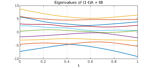
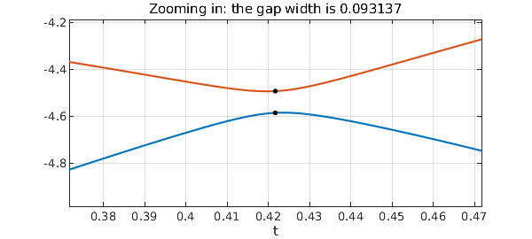
The 1st and 2nd curves have a very close near-crossing. We can find it like this:
E5 = E(:,1); E6 = E(:,2);
[minval,minpos] = min(E6-E5)
minval =
   0.093136973027921
minpos =
   0.421670169669245
Let's zoom in and mark the minimal gap in black:
axis([minpos-.05 minpos+.05 E5(minpos)-.4 E5(minpos)+.4])
title(['Zooming in: the gap width is ' num2str(minval)]), hold on
plot(minpos,E5(minpos),'.k','markersize',12)
plot(minpos,E6(minpos),'.k','markersize',12), hold off
References
-
P. Lax, Linear Algebra, Wiley, 1996.
-
J. von Neumann and E. Wigner, Über das Verhalten von Eigenwerten bei adiabatischen Prozessen, Physicalische Zeitschrift, 30 (1929), 467-470.