function Drum

The axisymmetric harmonic vibrations of a circular drum can be described by the ODE

$$ u''(r) + r^{-1} u'(r) = -\omega^2 u(r),~~ u'(0)=1, u(1)=0, $$

where $r$ is the radial coordinate and $\omega$ is the frequency of vibration. Only discrete positive values of $\omega$ are possible, corresponding to the eigenvalues of the differential equation.

We multiply the ODE through by $r$ to avoid a potential division by zero. This creates a generalized problem in the form $Au = \lambda Bu$.

r = chebfun('r',[0,1]);
A = chebop(0,1);
A.op = @(r,u) r*diff(u,2) + diff(u);
A.lbc = 'neumann'; A.rbc = 'dirichlet';
B = chebop(0,1);
B.op = @(r,u) r*u;

Then we find the eigenvalues with eigs. It turns out that the $\omega$ values are also zeros of the Bessel function $J_0$, which gives a way to valudate the results.

[V,D] = eigs(A,B);
[omega,ii] = sort(sqrt(-diag(D)));
omega
V = [V{:,ii'}];
err = omega - sort(roots( besselj(0,chebfun('r',[0 20])) ))

omega =
   2.404825557946273
   5.520078110504802
   8.653727912948732
  11.791534439018191
  14.930917708488634
  18.071063967910305
err =
   1.0e-09 *
   0.250494291975656
   0.218500773030428
   0.037726266555183
   0.003904432333002
   0.000854427639752
  -0.000625277607469

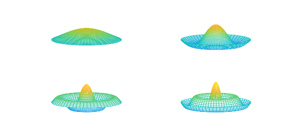
We also get the eigenfunctions, which gives a way to visualize deflections of the drums for pure frequencies.

V = V*diag(sign(V(0,:)));  % ensure V(0,k) > 0
[rr,tt] = meshgrid(linspace(0,1,40),linspace(0,2*pi,60));
for k = 1:4,
  subplot(2,2,k), mesh(rr.*cos(tt),rr.*sin(tt),repmat(V(rr(1,:),k),60,1))
  zlim([-1 3]),caxis([-3 3]), view(-33,20), axis off
end

If the drum instead has a variable density given by $\rho(r)$, the right- hand side of the original ODE becomes $-\omega^2\rho u$. In general, the connection to Bessel functions is broken, but we will not miss a beat using eigs.

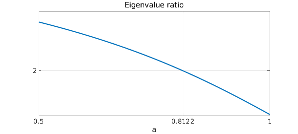
Constant density gives $\omega_2/\omega_1 = 2.2954$. Let's design a density so that $\omega_2/\omega_1 = 2$, a perfect octave. We will search among density functions of the form

$$ \rho(r) = 1 - a\sin(\pi r). $$

Here is a function that returns the ratio for any $a$.

function ratio = evratio(a)
  rho = 1 - a*sin(pi*r);
  B.op = @(r,u) r*rho*u;
  [V,D] = eigs(A,B,2,0);
  [omega,ii] = sort(sqrt(-diag(D)));
  V = [V{:,ii'}];
  ratio = omega(2)/omega(1);
end

Now, we create a chebfun to hit the target.

ratfun = chebfun(@evratio,[0.5,1]);
astar = find(ratfun==2)
clf, plot(ratfun), title('Eigenvalue ratio'), xlabel('a')
set(gca,'xtick',[0.5,astar,1],'ytick',[2],'xgrid','on','ygrid','on')

astar =
   0.812158808552563

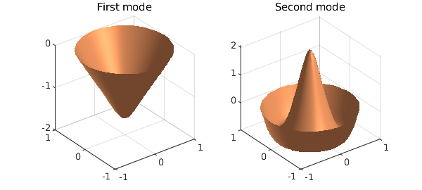
We compute the ratio at astar to verify the answer, and plot the eigenfunctions.

residual = evratio(astar) - 2
subplot(1,2,1), surfl(rr.*cos(tt),rr.*sin(tt),repmat(-V(rr(1,:),1),60,1))
shading interp, lighting phong, title('First mode')
subplot(1,2,2), surfl(rr.*cos(tt),rr.*sin(tt),repmat(-V(rr(1,:),2),60,1))
shading interp, lighting phong, title('Second mode')
colormap copper

residual =
    -3.648192858918264e-12

end

Couldn't create JOGL canvas--using painters
Couldn't create JOGL canvas--using painters
Couldn't create JOGL canvas--using painters
Couldn't create JOGL canvas--using painters
Couldn't create JOGL canvas--using painters
Couldn't create JOGL canvas--using painters
Couldn't create JOGL canvas--using painters
Couldn't create JOGL canvas--using painters
Couldn't create JOGL canvas--using painters
Couldn't create JOGL canvas--using painters
Couldn't create JOGL canvas--using painters
Couldn't create JOGL canvas--using painters
Couldn't create JOGL canvas--using painters