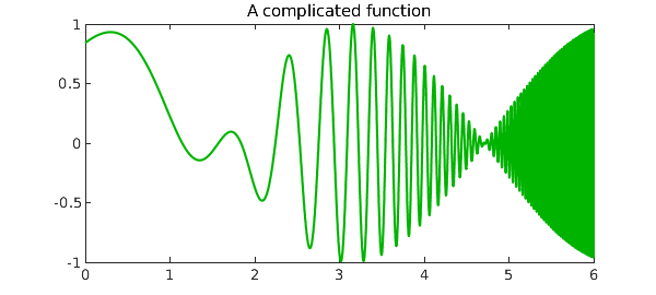
Here is the function $\cos(x)\sin(e^x)$ on the interval $[0,6]$:

tic, x = chebfun('x',[0 6]);
f = cos(x)*sin(exp(x));
length(f)
plot(f,'color',[0 .7 0])
title('A complicated function')

ans =
   551

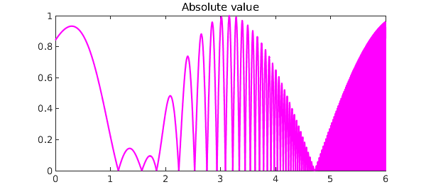
Here's its absolute value:

g = abs(f);
ax = [0 6 0 1];
plot(g,'m'), axis(ax)
title('Absolute value')

Here's the minimum of that function and $x/8$:

h = min(g,x/8);
plot(h), axis(ax)
title('Minimum with x/8')

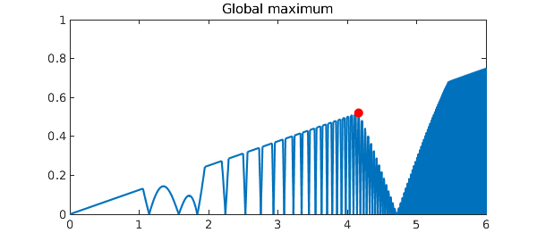
We can find the maximum over the interval $[0,5]$ like this:

MS = 'markersize';
[maxval,maxpos] = max(h{0,5})
hold on, plot(maxpos,maxval,'.r',MS,20)
title('Global maximum')

maxval =
   0.520496207016824
maxpos =
   4.164759283173317

Let's add all the local maxima to the plot:

[val,pos] = max(h,'local');
plot(pos,val,'.k',MS,10)
plot(maxpos,maxval,'.r',MS,20)
title('Local maxima')

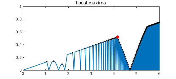
These computations showcase the fact that Chebfun optimization is global -- whether in the sense of finding a global extremum, or in the sense of globally finding all the local extrema.

They also showcase the treatment of discontinuities. To find extrema, Chebfun examines zeros of the derivative. In some cases those are points where the derivative is continuous and passes through zero. In others, like the black dot near $x=1$ in the plot above, they are points where the derivative jumps from positive to negative or vice versa.

Here is the time for this whole sequence of computations:

Total_time = toc

Total_time =
   5.092648000000000