LW = 'linewidth'; dom = [0 2*pi];

Consider the time-dependent PDE

$$ u_t = \mathcal{L}u, $$

on $[0,2\pi]\times[0,\infty)$, with a given periodic initial condition $u(x,0)$. We seek periodic solutions $u(x,t)$. If the operator $\mathcal{L}$ is semi-bounded, this problem is well-posed [1], and the unique solution is given by

$$ u(x,t) = e^{\mathcal{L}t}u(x,0). $$

Two examples of well-posed problems are the convection equation, $\mathcal{L}u=c(x)u_x$, and the heat equation, $\mathcal{L}u=u_{xx}$.

Consider first the convection equation

$$ u_t = c(x)u_x, $$

on $[0,2\pi]\times[0, 20]$, with $c(x)= -\frac{1}{5}-\sin^2(x-1)$, periodic boundary conditions, and initial condition $u(x,0)=\exp(-100(x-1)^2)$.

T = 20; dt = 0.5;
t = [0:dt:T];
c = chebfun(@(x) -(1/5 + sin(x-1).^2), dom);
L = chebop(@(x,u) c.*diff(u, 1), dom);
L.bc = 'periodic';
u0 = chebfun(@(x) exp(-100*(x-1).^2), dom);
u = expm(L, t, u0);
figure, waterfall(u, t, LW, 2)
view(10, 70), axis([0 2*pi 0 T 0 1])

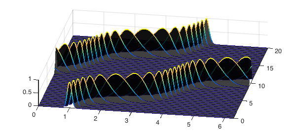
This example from [2] shows the propagation of the initial condition at variable speed, which remains coherent and clean.

Consider now the heat equation

$$ u_t = u_{xx}, $$

on $[0,2\pi]\times[0, 1]$, with periodic boundary conditions, and initial condition $u(x,0)=\sin(3x)$. We can solve it in Chebfun as follows with the expm command.

T = 1; dt = 0.05;
t = [0:dt:T];
L = chebop(@(u) diff(u, 2), dom);
L.bc = 'periodic';
u0 = chebfun(@(x) sin(3*x), dom);
u = expm(L, t, u0);
figure, waterfall(u, t, LW, 2)
view(10, 70), axis([0 2*pi 0 T -1 1])

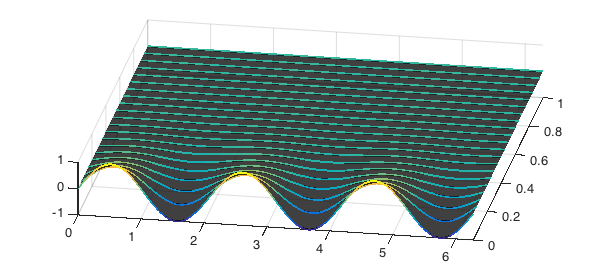
The diffusion has done its job: the solution at $T=1$ has very small amplitude.

norm(u{end}, inf)

ans =
     1.234098040878846e-04

References

1. J. S. Hesthaven, S. Gottlieb, and D. Gottlied, Spectral Methods for Time-Dependent Problems, Cambridge University Press, New York, 2007.

2. L. N. Trefethen, Spectral Methods in MATLAB, SIAM, Philadelphia, 2000.