1. Numerical integration over the disk
In studying cubature formulas, we needed to compute the integrals of products of Chebyshev polynomials $T_j(x) T_k(y)$ over the unit disk, like this one:
T8 = chebpoly(8); T16 = chebpoly(16);
s = linspace(-1,1,160); [xx,yy] = meshgrid(s,s);
ff = T8(xx).*T16(yy);
ff(xx.^2+yy.^2>1) = NaN;
contour(s,s,ff), axis equal off
hold on, plot(chebfun('exp(1i*x)',[0 2*pi]),'k'), hold off
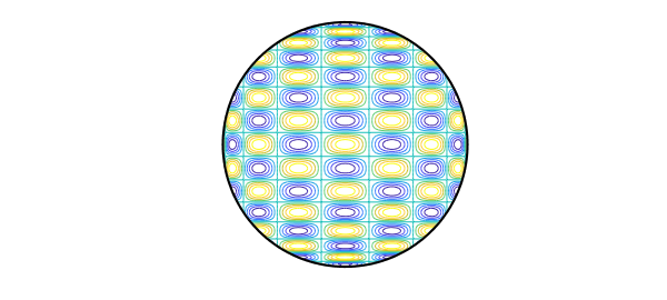
If $j$ or $k$ is odd, the integral is zero, but even if they are both even, to our surprise, we found that the integrals are still usually zero! In fact, a nonzero result only shows up if $j$ and $k$ differ by 0 or 2. Thus the function plotted above, for example, has integral exactly zero over the disk. This is not obvious.
Speaking in general, suppose we want to integrate a smooth function $f(r,t)$ numerically over the unit disk, where $r$ is radius and $t$ is angle. One could use Diskfun, but here, we use standard Chebfun. Let's assume that $f$ is defined by a function that accepts a scalar $r$ and a vector $t$, like this one:
f = @(r,t) 1 + 0*t;
Here is a numerical confirmation that the integral of $1$ is $\pi$:
format long
fr = @(r) r*sum(chebfun(@(t) f(r,t),[0,2*pi],'trig'));
I = sum(chebfun(@(r) fr(r),[0 1]))
Iexact = pi
I =
   3.141592653589793
Iexact =
   3.141592653589793
For the function $f(r,t) = r^2$, the integral is $\pi/2$:
f = @(r,t) r^2 + 0*t;
fr = @(r) r*sum(chebfun(@(t) f(r,t),[0,2*pi],'trig'));
I = sum(chebfun(@(r) fr(r),[0 1]))
Iexact = pi/2
I =
   1.570796326794897
Iexact =
   1.570796326794897
For the function $f(r,t) = r^2 \cos^2(t)$, the integral is $\pi/2$:
f = @(r,t) r^2*cos(t).^2;
fr = @(r) r*sum(chebfun(@(t) f(r,t),[0,2*pi],'trig'));
I = sum(chebfun(@(r) fr(r),[0 1]))
Iexact = pi/4
I =
   0.785398163397448
Iexact =
   0.785398163397448
2. Numerical integration of products of Chebyshev polynomials
What about those products of Chebyshev polynomials? Here is a matrix showing the numerically computed integrals for $k = 0,2,4,6,8,10$. As claimed above, the matrix is tridiagonal.
tic
I = zeros(6);
format short
for j = 0:2:10
  Tj = chebpoly(j);
  for k = 0:2:j
    Tk = chebpoly(k);
    f = @(r,t) Tk(r*cos(t)).*Tj(r*sin(t));
    fr = @(r) r*sum(chebfun(@(t) f(r,t),[0,2*pi],'trig'));
    I(1+j/2,1+k/2) = sum(chebfun(@(r) fr(r),[0 1]));
  end
end
I = I + tril(I,-1)'
time_elapsed_in_seconds = toc
I =
    3.1416   -1.5708   -0.0000    0.0000   -0.0000    0.0000
   -1.5708    0.5236    0.2618    0.0000   -0.0000   -0.0000
   -0.0000    0.2618   -0.1047   -0.1571    0.0000   -0.0000
    0.0000    0.0000   -0.1571    0.0449    0.1122    0.0000
   -0.0000   -0.0000    0.0000    0.1122   -0.0249   -0.0873
    0.0000   -0.0000   -0.0000    0.0000   -0.0873    0.0159
time_elapsed_in_seconds =
    3.7174
3. Analytic expressions for the integrals
Let $I_{jk}$ denote the integral of $T_j(x) T_k(y)$ over the unit disk. The following explicit formulas derived by the first author (details not reported here) give the integrals:
$$ I_{00} = \pi, $$
$$ I_{02} = I_{20} = -{\pi\over 2}, $$
$$ I_{kk} = {\pi (-1)^{k/2} \over 2 - 2k^2} \quad \hbox{($k$ even, $k\ge 2$)}, $$
$$ I_{k,k+2} = I_{k+2,k} = {\pi (-1)^{1+k/2} \over 4k + 4} \quad \hbox{($k$ even, $k\ge 2$)}, $$
In all other cases $I_{jk} = 0$.
Using these formulas, we can reproduce the matrix above as follows:
I = zeros(6);
I(1,1) = pi;
I(2,1) = -pi/2;
for k = 2:2:10
  I(1+k/2,1+k/2) = pi*(-1)^(k/2)/(2-2*k^2);
end
for k = 2:2:8
  I(2+k/2,1+k/2) = -pi*(-1)^(k/2)/(4*k+4);
end
I = I + tril(I,-1)'
I =
    3.1416   -1.5708         0         0         0         0
   -1.5708    0.5236    0.2618         0         0         0
         0    0.2618   -0.1047   -0.1571         0         0
         0         0   -0.1571    0.0449    0.1122         0
         0         0         0    0.1122   -0.0249   -0.0873
         0         0         0         0   -0.0873    0.0159
4. Application to integration of general functions
The results of the last section imply that there is an immediate way to compute the integral of a chebfun2 over a disk: just take the appropriate linear combination of its bivariate Chebyshev coefficients. After this example was initially written, we developed this idea into a Chebfun2 sumdisk command. See the example "Sumdisk for integration over a disk".