12.1 What is a chebfun2?
Chebfun2 is the part of Chebfun that deals with functions of two variables defined on a rectangle $[a,b]\times[c,d]$. Just like Chebfun in 1D, it is an extremely convenient tool for all kinds of computations including algebraic manipulation, optimization, integration, and rootfinding. It also extends to vector-valued functions of two variables, so that one can perform vector calculus.
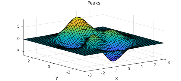
For example, here is a test function that has been part of MATLAB for many years. MATLAB represents the "peaks" function by a $49\times 49$ matrix:
peaks
z =  3*(1-x).^2.*exp(-(x.^2) - (y+1).^2) ...
   - 10*(x/5 - x.^3 - y.^5).*exp(-x.^2-y.^2) ...
   - 1/3*exp(-(x+1).^2 - y.^2)
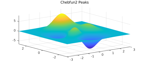
The same function is available as a chebfun2 in the Chebfun2 gallery:
f = cheb.gallery2('peaks');
plot(f), axis tight, title('Chebfun2 Peaks')
In Chebfun we can do all sorts of things with functions to a high accuracy, such as evaluate them
f(0.5,0.5)
ans =
   0.375375578848315
or compute their maxima,
max2(f)
ans =
   8.106213589442337
A chebfun2, with a lower-case "c", is a MATLAB object, the 2D analogue of a chebfun. The syntax for chebfun2 objects is similar to the syntax for matrices in MATLAB, and Chebfun2 objects have many MATLAB commands overloaded. For instance, trace(A) returns the sum of the diagonal entries of a matrix $A$ and trace(f) returns the integral of $f(x,x)$ when $f$ is a chebfun2.
Chebfun2 builds on Chebfun's univariate representations and algorithms. Algorithmic details are given in [Townsend & Trefethen 2013b] and mathematical underpinnings in [Townsend & Trefethen 2014]. For more information, see Section 12.8.
12.2 What is a chebfun2v?
Chebfun2 can represent scalar-valued functions, such as $\exp(x+y)$, and vector-valued functions, such as $[\exp(x+y);\cos(x-y)]$. A vector-valued function is called a chebfun2v, and chebfun2v objects are useful for computations of vector calculus. For information about chebfun2v objects and vector calculus, see Chapters 15 and 16 of this guide.
12.3 Constructing chebfun2 objects
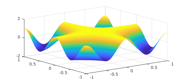
A chebfun2 can be constructed by supplying the Chebfun2 constructor with a bivariate function handle or string. The default rectangular domain is $[-1,1]\times [-1,1]$. (An example showing how to specify a different domain is given in section 6.) For example, here we construct and plot a chebfun2 representing $\cos(2\pi xy)$ on $[-1,1]\times[-1,1]$.
f = chebfun2(@(x,y) cos(2*pi*x.*y));
We could equally well have constructed chebfun2 objects for the variables $x$ and $y$ first and then computed $f$ from these:
x = chebfun2(@(x,y) x);
y = chebfun2(@(x,y) y);
f = cos(2*pi*x.*y);
There's also a shortcut cheb.xy to constructing these objects x and y, so we could also have executed
cheb.xy
f = cos(2*pi*x.*y);
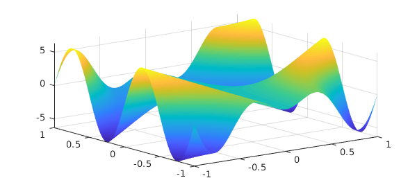
Here is a plot of $f$:
plot(f), zlim([-2 2])
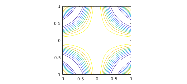
Along with plot, there are also commands contour and surf for displaying a chebfun2. Here is a contour plot of $f$:
contour(f), axis square
One way to find the rank of the approximant used to represent $f$, discussed in Section 8.8, is like this:
length(f)
ans =
    11
Alternatively, more information can be given by displaying the chebfun2 object:
f
f =
   chebfun2 object
       domain                 rank       corner values
[  -1,   1] x [  -1,   1]       11     [   1    1    1    1]
vertical scale =   1
The corner values are the values of the chebfun2 at $(-1,-1)$, $(-1,1)$, $(1,-1)$, and $(1,1)$, in that order. The vertical scale is used by operations to aim for close to machine precision relative to that number.
12.4 Basic operations
Once we have a chebfun2, we can compute quantities such as its definite double integral:
sum2(f)
ans =
   0.902823333580281
This matches well the exact answer obtained by calculus, which is $(2/\pi)\hbox{Si}(2\pi)$:
exact = 0.9028233335802806267957003779
exact =
   0.902823333580281
We can also evaluate a chebfun2 at a point $(x,y)$, or along a line. When evaluating along a line a chebfun is returned because the answer is a function of one variable.
Evaluation at a point:
x = 2*rand - 1; y = 2*rand - 1;
f(x,y)
ans =
  -0.997677434419261
Evaluation along the line $y = \pi/6$:
f(:,pi/6)
ans =
   chebfun row (1 smooth piece)
       interval       length     endpoint values
[      -1,       1]       23     -0.99    -0.99
vertical scale =   1
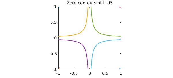
There are plenty of other questions that may be of interest. For instance, what are the zero contours of $f(x,y) - .95$?
r = roots(f-.95);
plot(r), axis([-1 1 -1 1])
axis square, title('Zero contours of f-.95')
What is the partial derivative $\partial f/\partial y$?
fy = diff(f,1,1);
plot(fy)
The syntax for the diff command can cause confusion because we are following the matrix syntax in MATLAB. Chebfun2 also offers the more easily remembered diffx(f,k) and diffy(f,k), which differentiate $f(x,y)$ $k$ times with respect to the first and second variable, respectively.
What is the mean value of $f$ on $[-1,1]\times[-1,1]$?
mean2(f)
ans =
   0.225705833395070
12.5 Chebfun2 methods
There are over 100 methods that can be applied to chebfun2 objects. For a complete list type:
methods chebfun2
Methods for class chebfun2:

abs                   horzcat               quiver3
biharm                imag                  rank
biharmonic            integral              rdivide
cdr                   integral2             real
chebcoeffs2           isPeriodicTech        restrict
chebfun2              isempty               roots
chebpolyplot          isequal               roots0
chebpolyplot2         isreal                rootsFeb19
chebpolyval2          iszero                rootsclean
chol                  jacobian              rootsfine
coeffs2               lap                   rootsnew
complex               laplacian             sample
compose               ldivide               sampleTest
conj                  length                simplify
constructor           log                   sin
contour               lu                    singleSignTest
contourf              max                   sinh
cos                   max2                  size
cosh                  mean                  sph2cart
ctranspose            mean2                 sphere
cumprod               median                sqrt
cumsum                mesh                  squeeze
cumsum2               min                   std
dblquad               min2                  std2
diag                  minandmax2            subsref
diff                  minandmax2est         sum
diffx                 minus                 sum2
diffy                 mldivide              sumdisk
discriminant          mrdivide              surf
disp                  mtimes                surface
display               norm                  surfacearea
domainCheck           normalizePivots       svd
domainarea            normalizeRowsAndCols  tan
eig                   pivotplot             tand
ellipsoid             pivots                tanh
end                   plot                  times
exp                   plotcoeffs            trace
explain               plotcoeffs2           transpose
feval                 plus                  uminus
fevalm                pol2cart              uplus
flipdim               poldec                vertcat
fliplr                potential             volt
flipud                power                 vscale
fred                  prod                  waterfall
get                   qr
grad                  quad2d
gradient              quiver

Static methods:

chebpts2              paduaVals2coeffs
coeffs2vals           poisson
outerProduct          vals2coeffs
Most of these commands have been overloaded from MATLAB. More information about a Chebfun2 command can be found with help:
help chebfun2/max2
 MAX2   Global maximum of a CHEBFUN2.
    Y = MAX2(F) returns the global maximum of F over its domain.

    [Y, X] = MAX2(F) returns the global maximum in Y and its location X.

   This command may be faster if the OPTIMIZATION TOOLBOX is installed.

  See also MIN2, MINANDMAX2.
12.6 Composition of chebfun2 objects
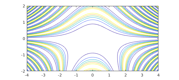
New chebfun2 objects can be constructed from existing ones by composing them with operations such as +, -, .*, and .^. For example,
x = chebfun2(@(x,y) x, [-4 4 -2 2]);
y = chebfun2(@(x,y) y, [-4 4 -2 2]);
f = 1./( 2 + cos(.25 + x.^2.*y + y.^2) );
contour(f), axis equal
12.7 Analytic functions
An analytic function $f(z)$ can be thought of as a complex-valued function of two real variables, $f(x,y) = f(x+iy)$. If the Chebfun2 constructor is given an anonymous function with one argument, it assumes that argument is a complex variable. For instance,
f = chebfun2(@(z) sin(z));
f(1+1i), sin(1+1i)
ans =
  1.298457581415977 + 0.634963914784736i
ans =
  1.298457581415977 + 0.634963914784736i
These functions can be visualised by using a technique known as phase portrait plots. Given a complex number $z = re^{i\theta}$, the phase $e^{i\theta}$ can be represented by a colour. We follow Wegert's colour recommendations [Wegert 2012], using red for a phase $i$, then yellow, green, blue, and violet as the phase moves clockwise around the unit circle. For example,
f = chebfun2(@(z) sin(z)-sinh(z),2*pi*[-1 1 -1 1]);
plot(f)
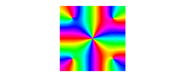
Many properties of analytic functions can be visualised by these types of plots, such as the location of zeros and their multiplicities. Can you work out the multiplicity of the root at $z=0$ from this plot? For another example, try cheb.gallery2('airycomplex').
Since Chebfun2 only represents smooth functions, a trick is required to draw pictures like these for functions with poles [Trefethen 2013]. For functions with branch points or essential singularities, it is currently not possible in Chebfun2 to draw phase plots.
12.8 Chebfun2 low rank approximations
Chebfun2 exploits the observation that many functions of two variables can be well approximated by low rank approximants. A rank $1$ function, also known as separable, is of the form $u(y)v(x)$, and a rank $k$ function is one that can be written as the sum of $k$ rank $1$ functions. Smooth functions tend to be well approximated by functions of low rank. Chebfun2 determines low rank function approximations automatically by means of an algorithm that can be viewed as an iterative application of Gaussian elimination with complete pivoting [Townsend & Trefethen 2013]. The underlying function representations are related to work by Carvajal, Chapman and Geddes [Carvajal, Chapman, & Geddes 2008] and others including Bebendorf [Bebendorf 2008], Hackbusch, Khoromskij, Oseledets, and Tyrtyshnikov. For further aspects of low-rank representations see [Trefethen 2017] and [Beckermann and Townsend 2019].
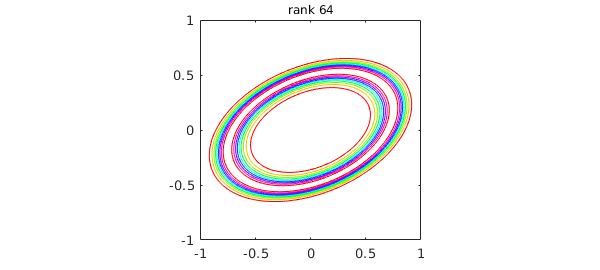
Here is an example adapted from [Townsend & Trefethen 2013] and cheb.gallery2('smokering'). The function $$ f(x,y) = \exp( -40(x^2-xy+2y^2 - 1/2)^2) $$ has the shape of an elliptical ring in the unit square, and Chebfun2 represents it by an approximation of reasonably high rank:
ff = @(x,y) exp(-40*(x.^2 - x.*y + 2*y.^2 - 1/2).^2);
f = chebfun2(ff);
levels = 0.1:0.1:0.9;
contour(f,levels), axis([-1 1 -1 1]), axis square
title(['rank ' int2str(length(f))],'fontsize',12)
To illustrate the nature of low-rank approximations, rather than letting Chebfun2 determine the rank adaptively, we can force it to take ranks $1,2,\dots ,9$. Here are the results, plotted with black level curves at heights $0.2,0.4,0.6,0.8$:
levels = 0.2:0.2:0.8;
clf
for k = 1:9
    axes('position',[.03+.33*mod(k-1,3) .67-.3*floor((k-1)/3) .28 .28])
    contour(chebfun2(ff,k),levels,'k')
    xlim([-1 1]), axis equal, axis off
end
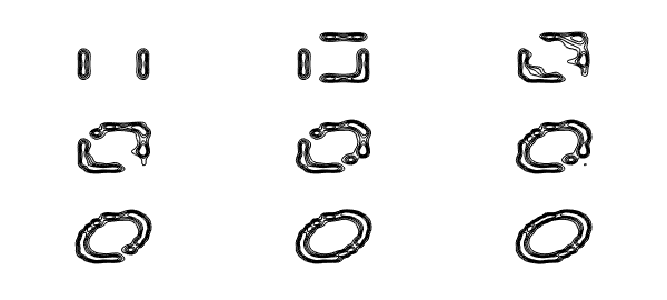
For this function, "plotting accuracy" is achieved approximately at rank 16; the remaining terms are then required to get from 2-3 digits to 15.
12.9 References
[Bebendorf 2008] M. Bebendorf, Hierarchical Matrices: A Means to Efficiently Solve Elliptic Boundary Value Problems, Springer, 2008.
[Beckermann & Townsend 2019] "Bounds on the singular values of matrices with displacement structure", SIAM Rev. 61 (2019), 319--344.
[Carvajal, Chapman, & Geddes 2008] O. A. Carvajal, F. W. Chapman and K. O. Geddes, "Hybrid symbolic-numeric integration in multiple dimensions via tensor-product series", Proceedings of ISSAC'05, M. Kauers, ed., ACM Press, 2005, 84-91.
[Townsend & Trefethen 2013] A. Townsend and L. N. Trefethen, "Gaussian elimination as an iterative algorithm", SIAM News, March 2013.
[Townsend & Trefethen 2013b] A. Townsend and L. N. Trefethen, "An extension of Chebfun to two dimensions", SIAM Journal on Scientific Computing, 35 (2013), C495-C518.
[Townsend & Trefethen 2014] A. Townsend and L. N. Trefethen, "Continuous analogues of matrix factorizations", Proceedings of the Royal Society A 471 (2014) 20140585.
[Trefethen 2013] L. N. Trefethen, "Phase Portraits for functions with poles", http://www.chebfun.org/examples/complex/PortraitsWithPoles.html.
[Trefethen 2017] L. N. Trefethen, "Cubature, approximation, and isotropy in the hypercube", SIAM Rev. 59 (2017), 469--491.
[Wegert 2012] E. Wegert, Visual Complex Functions: An Introduction with Phase Portraits, Birkhauser/Springer, 2012.