Here is the matrix from the Chebfun2 example 'Hello World' (see http://www.chebfun.org/examples/fun/HelloWorld.html).
A=zeros(15,40);
A(2:9,2:3)=1; A(5:6,4:5)=1;A(2:9,6:7)=1; A(3:10,10:11)=1;
A(3:4,10:15)=1; A(6:7,10:15)=1; A(9:10,10:15)=1; A(4:11,18:19)=1;
A(10:11,18:24)=1; A(5:12,26:27)=1; A(11:12,26:31)=1;
A(6:13,34:35)=1; A(6:13,38:39)=1; A(6:7,36:37)=1; A(12:13,36:37)=1;
We pad it with zeros to size $40\times 40$ and add a third dimension:
A = [zeros(14,40); A; zeros(11,40)];
A = fliplr(flipud(A));
B = zeros(40,40,40);
for k = 18:21
    B(k,:,:) = A;
end
B is now a $40\times 40\times 40$ tensor whose entries are all zeros and ones.
A chebfun3 is normally constructed from a function handle for a function $f(x,y,z)$. It is also possible to do it from discrete data, and we can specify that this is to be interpreted as living on an equispaced grid:
f = chebfun3(B, 'equi');
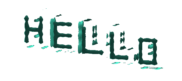
Let's plot the result:
f = permute(f, [1, 3, 2]);
isosurface(f, 0.5)
view([-2.5, -1, 0.4]), camlight, axis off, axis equal

From a function approximation point of view, this is most definitely not well resolved! Readers may have fun calling isosurface(f) to explore different levels with a slider. For example, here is what we get at level $-0.1$, a value below all of the input data:
isosurface(f, -0.1)
view([-2.5, -1, 0.4]), camlight, axis off, axis equal
In this example we approximated the discrete HELLO tensor using the 'equi' flag, leading to a trivariate Chebyshev representation associated with equispaced data. A more straightforward approach mathematically would be to regard the tensor as triply periodic and form a chebfun3 from it with the 'trig' flag instead. Experiments show that if this is done, the pictures look similar.