For a couple of years Chebfun has had a command conformal for computing a conformal map of a smooth simply connected region onto the unit disk, and now there is a companion command conformal2 for mapping a smooth doubly-connected region onto a circular annulus. The conformal modulus, which is the ratio of the inner to outer radii of the annulus, is determined in the process.

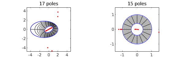
For example, here we map a region $\Omega$ bounded by two ellipses to the annulus $A_\rho$ with $\rho \approx 0.409705$.

circle = chebfun('exp(1i*pi*t)','trig');
ellipse = real(circle) + .6i*imag(circle);
C1 = 3*ellipse - 1; C2 = exp(.5i)*ellipse;
tic, [f, finv, rho] = conformal2(C1,C2,'plots'); toc
rho

Elapsed time is 3.344638 seconds.
rho =
   0.409705344001635

Here we do it again but to 12-digit accuracy instead of the default 6 digits:

tic, [f, finv, rho] = conformal2(C1,C2,'plots','tol',1e-12); toc
rho

Elapsed time is 7.900462 seconds.
rho =
   0.409705344001634

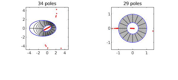
As with the simply-connected conformal, the red dots show poles associated with the numerical representations of these maps. The objects f and finv are function handles corresponding to AAA rational approximations of the maps from $\Omega$ to $A_\rho$ and from $A_\rho$ to $\Omega$, respectively. The accuracy in much of the domain is actually better than 12 digits, as we verify by mapping the points $1, i$ back and forth:

z = [1 1i];
finv(f(z))

ans =
  Column 1
  1.000000000000036 - 0.000000000000013i
  Column 2
  0.000000000000006 + 0.999999999999992i

These rational representations are fantastically efficient. We can map a million points back and forth in 1 second.

z = 1 + .1*rand(1e6,1) + .1i*rand(1e6,1);
tic, finv(f(z)); toc

Elapsed time is 0.515038 seconds.

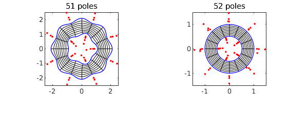
Here is a wigglier example.

circle = chebfun('exp(1i*pi*t)','trig');
C1 = circle*chebfun('2+.1*cos(8*pi*t)','trig');
C2 = circle*chebfun('1+.1*cos(5*pi*t)','trig');
tic, [f, finv, rho] = conformal2(C1,C2,'plots'); toc
rho

Elapsed time is 3.736870 seconds.
rho =
   0.515907564661642

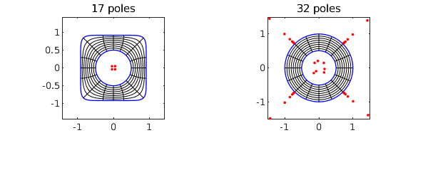
Here is a "hyperellipse" enclosing a disk. Note how we define the hyperellipse via a level curve of a chebfun2.

F = chebfun2(@(x,y) x.^8 + y.^8);
C1 = roots(F-.5); C2 = .5*circle;
tic, [f, finv, rho] = conformal2(C1,C2,'plots'); toc
rho

Elapsed time is 3.156300 seconds.
rho =
   0.506114112297563

The algorithm used by conformal2 consists of solving a Laplace problem (computing a Green's function) by Laurent expansion with least-squares collocation on the boundary, as described in [2]. A key part of this is the use of Vandermonde with Arnoldi orthogonalization [1], which is available with the Chebfun commands VAorthog and VAeval. (The latter is actually not needed for this application because the AAA rational functions do the evaluation instead.)

Both conformal and conformal2 are restricted in their applicability to smooth domains. As described in [2], related algorithms have been developed for regions with corners, but these are not currently available in Chebfun.

[1] P. D. Brubeck, Y. Nakatsukasa, and L. N. Trefethen, Vandermonde with Arnoldi, SIAM Review 63 (2021), 405-415.

[2] L. N. Trefethen, Numerical conformal mapping with rational functions, Computational Methods and Function Theory (2020), 1-19.