One of the new features of Chebfun version 5 is the ability to create chebfuns of smooth periodic functions using Fourier series. This example introduces and demonstrates some of the functionality of this new tool.
Construction and comparison
Fourier-based chebfuns, or "trigfuns" as we like to refer to them, can be created with the use of the 'trig' flag in the chebfun constructor. For, example, the function $f(x) = \cos(8\sin(x))$ for $-\pi \leq x \leq \pi$ can be constructed as follows:
dom = [-pi,pi];
f = chebfun(@(x) cos(8*sin(x)),dom,'trig')
plot(f);
f =
   chebfun column (1 smooth piece)
       interval       length     endpoint values trig
[    -3.1,     3.1]       61         1        1
vertical scale =   1
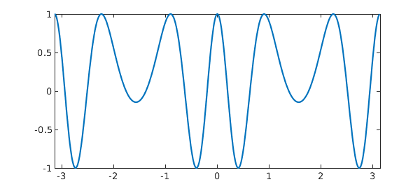
Here $f$ is represented to machine precision using a Fourier interpolant rather than a Chebyshev interpolant. The displayed information for $f$ above shows that it is of length 61, meaning that $f$ is resolved to machine precision using 61 samples, or $(61-1)/2=30$ (complex) Fourier modes. These coefficients can be displayed graphically by
plotcoeffs(f), ylim([1e-18 1])
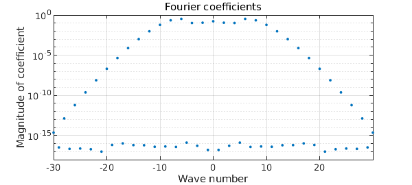
Since $f$ is smooth and periodic, a Fourier representation requires fewer terms than a Chebyshev representation of $f$ to reach machine precision. We can check this by constructing $f$ without the 'trig' flag:
f_cheby = chebfun(@(x) cos(8*sin(x)),dom)
f_cheby =
   chebfun column (1 smooth piece)
       interval       length     endpoint values
[    -3.1,     3.1]      103         1        1
vertical scale =   1
The ratio of length of the Chebyshev series to the Fourier series should be approximately $\pi/2$ since the former has a resolution power of $\pi$ points per wavelength and the latter of 2 points per wavelength. We can check this numerically as
ratio = length(f_cheby)/length(f)
theoretical = pi/2
ratio =
   1.688524590163935
theoretical =
   1.570796326794897
Trying to construct a trigfun from a non-periodic or non-smooth function will typically result in a warning being issued and an "unhappy" trigfun, as illustrated for the unit step function below:
f = chebfun(@(x) 0.5*(1+sign(x)),dom,'trig')
plot(f);
Warning: Function not resolved using 65536 pts. Have you tried a non-trig
representation?
f =
   chebfun column (1 smooth piece)
       interval       length     endpoint values trig
[    -3.1,     3.1]    65536       0.5      0.5
vertical scale =   1
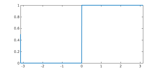
The length of $f$ is 65536, which is the maximum number of samples used in the construction process to try to resolve $f$. The famous Gibbs phenomenon can be seen near the discontinuity in the plot of $f$. Chebfun can be used to represent this function in non-periodic mode (i.e. using Chebyshev series) with the option of splitting on:
f = chebfun(@(x) 0.5*(1+sign(x)),dom,'splitting','on')
f =
   chebfun column (2 smooth pieces)
       interval       length     endpoint values
[    -3.1,       0]        1         0        0
[       0,     3.1]        1         1        1
vertical scale =   1    Total length = 2
Splitting is not an option for trigfuns.
Basic operations
Many Chebfun operations can also be applied directly to a trigfun. Some of these basic operations are illustrated in the examples below.
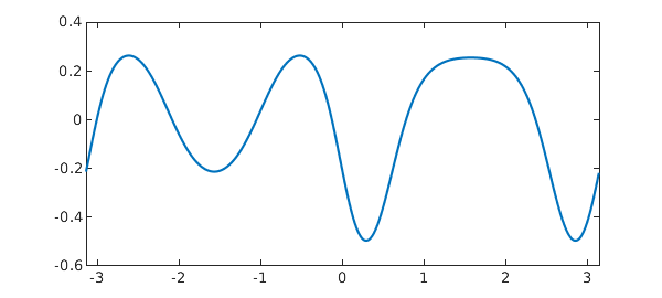
Addition, subtraction, multiplication, division, and function composition can all be directly applied to a trigfun. However one should be aware that operation should result in a smooth and periodic function. (If not, it will be converted to a nonperiodic chebfun.) The following example illustrates some of these operations:
g = chebfun(@(x) sin(x),dom,'trig');
f = tanh(cos(1+2*g)^2)-0.5
plot(f)
f =
   chebfun column (1 smooth piece)
       interval       length     endpoint values trig
[    -3.1,     3.1]      161     -0.22    -0.22
vertical scale = 0.5
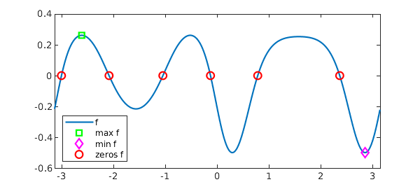
The max, min, and roots of $f$ can be computed by
[maxf,xmaxf] = max(f);
[minf,xminf] = min(f);
rootsf = roots(f);
maxf
minf
rootsf
maxf =
   0.261594155955765
minf =
  -0.500000000000000
rootsf =
  -3.009212218006482
  -2.090420462897022
  -1.051172190692770
  -0.132380435583317
   0.779312428506054
   2.362280225083739
These can be visualized as
plot(f), hold on
plot(xmaxf,maxf,'gs',xminf,minf,'md',rootsf,0*rootsf,'ro')
legend('f','max f','min f','zeros f','location','southwest')
hold off;
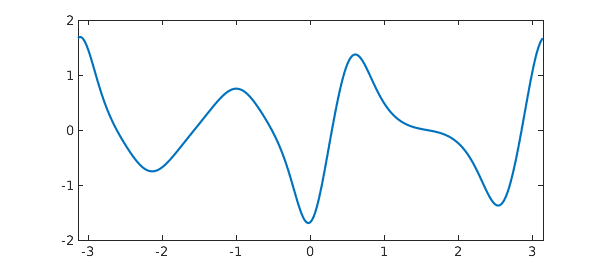
The derivative of $f$ is computed using diff:
df = diff(f);
plot(df)
and the definite integral is computed using sum:
intf = sum(f)
intf =
  -0.074010812957415
Complex-valued trigfuns are also possible. For example:
f = chebfun(@(x) 1i*(13*cos(x)-5*cos(2*x)-2*cos(3*x)-cos(4*x)) + ...
                 16*sin(x)^3, dom, 'trig')
plot(f), axis equal
f =
   chebfun column (1 smooth piece)
       interval       length     endpoint values trig
[    -3.1,     3.1]        9     complex values
vertical scale =  17
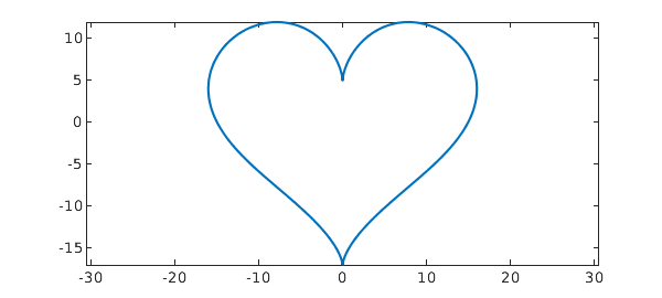
The area enclosed by this curve can be computed as
area_heart = abs(sum(real(f)*diff(imag(f))))
area_heart =
     5.654866776461628e+02
According to [1], the true area enclosed is $180\pi$. The relative error in the computation above is then
err = (area_heart - 180*pi)/(180*pi)
err =
     0
The convolution of two smooth periodic functions can be computed using the circconv (circular convolution) function. The example below demonstrates this function in combination with the additional feature that allows trigfuns to be constructed from function values. The latter is demonstrated first:
rng('default'), rng(0)
n = 201;
x = trigpts(n);
func_vals = exp(sin(2*pi*x)) + 0.05*randn(n,1);
f = chebfun(func_vals,dom,'trig')
f =
   chebfun column (1 smooth piece)
       interval       length     endpoint values trig
[    -3.1,     3.1]      201         1        1
vertical scale = 2.8
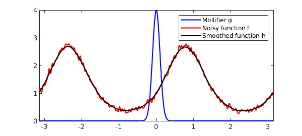
Here $f$ interpolates the noisy func_vals at 201 equally spaced points from $[-\pi,\pi)$ using the Fourier basis. The high frequencies in this function can be smoothed by convolving it with a mollifier, in this case a (normalized) Gaussian with variance 0.1.
sigma = 0.1;
g = chebfun(@(x) 1/(sigma*sqrt(2*pi))*exp(-0.5*(x/sigma)^2),dom,'trig');
Note that the resulting respresentation of $g$ is actually the periodic extension of the Gaussian over $[-\pi,\pi]$. The convolution of $f$ and $g$ is computed and visualized using
h = circconv(f,g);
plot(g,'b'), hold on
plot(f,'r'), plot(h,'k')
legend('Mollifier g','Noisy function f','Smoothed function h');
hold off;
References
- Mathworld Heart Curve: http://mathworld.wolfram.com/HeartCurve.html