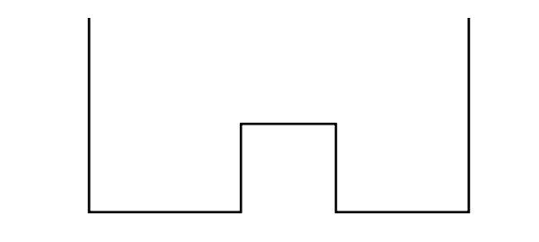
A well-known problem in quantum mechanics is the calculation of eigenstates of a potential with the shape of a "double well". Specifically, consider a potential function $V(x)$ defined on $[-1,1]$ by
$$ V(x) = 1.5, ~ x \in [-.2,.3], $$
and zero otherwise. We seek eigenmodes of the steady-state Schroedinger equation associated with this potential, specifically, functions $u(x)$ satisfying
$$ -0.007u''(x) + V(x)u(x) = \lambda u(x),~~ u(-1) = u(1) = 0 $$
for some constant $\lambda$.
We can sketch the potential like this:
plot([-1 -1 -.2 -.2 .3 .3 1 1],[3.3 0 0 1.5 1.5 0 0 3.3],'k','linewidth',2)
axis([-1.1 1.1 -.05 3.3]), axis off, hold on
Let's compute the first 12 eigenvalues and eigenfunctions:
tic
x = chebfun('x');
V = 1.5*(abs(x-0.05)<0.25);
L = chebop(-1,1);
L.op = @(x,u) -0.007*diff(u,2) + V*u;
L.bc = 0;
neigs = 12;
[EV,D] = eigs(L,neigs);
disp(diag(D)), toc
   0.091480998228306
   0.116757122005294
   0.363909308598088
   0.463167687393423
   0.808941736700779
   1.021145960789530
   1.390812031498700
   1.652575851342681
   1.871230031210215
   2.174488704532026
   2.533176594994659
   2.924094539796362
Elapsed time is 1.682039 seconds.
Physicists like to plot the eigenmodes shifted up by an amount equal to the eigenvalue:
colors = [1 0 0; 0 .8 0; .9 .9 0; 0 0 1; 1 0 1; 0 .8 1];
for j = 1:neigs
  v = EV(:,j)/15; d = D(j,j);
  if max(v)<-min(v), v = -v; end
  plot(d+v,'color',colors(1+mod(j-1,6),:))
end
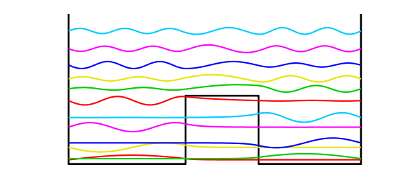
There is a great deal of such physics in such pictures. The lower eigenmodes correspond to particles trapped on one side or the other, with a state function decreasing exponentially within the barrier. At higher energies the particles are not localized.
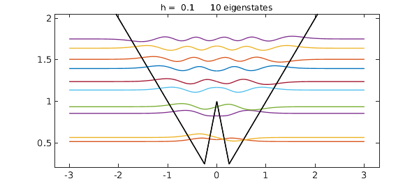
The Chebfun command quantumstates allows one to carry out explorations like these much more easily.
clf, x = chebfun('x',[-3,3])
V = max(abs(x),1-3*abs(x));
quantumstates(V)
x =
   chebfun column (1 smooth piece)
       interval       length     endpoint values
[      -3,       3]        2        -3        3
vertical scale =   3
Couldn't create JOGL canvas--using painters
Couldn't create JOGL canvas--using painters
ans =
   0.519275627855281
   0.568122999844246
   0.857289324405055
   0.936834938835163
   1.137321404215857
   1.238731857340433
   1.395322337063320
   1.505801742485166
   1.638922632407592
   1.750303602924204
For more information on problems like these, see chapter 6 of Exploring ODEs, freely available at people.maths.ox.ac.uk/trefethen/ExplODE/.