[revised July 2019]
1. Symmetric matrix
The Rayleigh quotient iteration (RQI) is a well-known algorithm for computing an eigenpair of a matrix $A$ (symmetric or nonsymmetric). Using an approximate $\tilde\lambda$ and approximate eigenvector $\tilde x$ (normalized by $|\tilde x|_2=1$), it updates the approximate eigenvector via one step of the shifted-and-inverted power method, $\tilde x:=(A-\tilde\lambda I)^{-1}\tilde x$, which is computed by solving a linear system (then normalized again). The approximate eigenvalue is then updated via the Rayleigh quotient $\tilde\lambda = \tilde x^\ast A\tilde x$. Under mild assumptions, by repeating the process, $\tilde x$ converges to an eigenvector, usually to the one corresponding to the eigenvalue that the initial $\tilde\lambda$ is closest to. The convergence of RQI is known to be asymptotically cubic when $A$ is symmetric [1, Sec. 4.6], and otherwise quadratic.
Here is an example showing cubic convergence for a random symmetric $10\times 10$ matrix. (Note that we sacrifice some efficiency in computing $Au$ in the residual computation for the sake of clarity. This could easily be avoided.)
rng(10)                                      % choose a random number seed
tol = 1e-10;
n = 10;
A = randn(n); A = A'+A;                      % symmetric matrix
I = eye(size(A));                            % identity

% Initial guesses:
disp('lam:')
lam = A(end,end); disp(lam)                  % seek eigenvalue near lam
u = rand(n,1);  u = u/norm(u);               % random guess
res = norm(A*u - lam*u)/norm(A*u);           % initial residual

% Rayleigh quotient iteration:
while ( res(end) > tol )
    u = (A - lam*I)\u; u = u/norm(u);        % core RQI
    lam = u'*A*u; disp(lam)                  % update Rayleigh quotient
    res = [res; norm(A*u-lam*u)/norm(A*u)];  % store residual
end
res
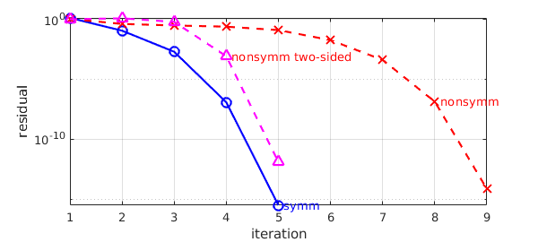
lam:
   3.290604172428599
   3.147338430697157
   3.125420718374708
   3.125374676595397
   3.125374676595200
res =
   1.344387798598789
   0.115727317111612
   0.002003341134186
   0.000000120617185
   0.000000000000000
2. Nonsymmetric matrix
Next let's try a nonsymmetric matrix. The convergence becomes quadratic.
A = randn(n);                                 % nonsymmetric matrix
% Initial guesses:
disp('lam:')
lam = A(end,end); disp(lam)                   % seek eigenvalue near lam
u = rand(n,1)+1i*randn(n,1); u = u/norm(u);   % random guess (eigval can be complex)
res2 = norm(A*u - lam*u)/norm(A*u);           % initial residual

% Rayleigh quotient iteration:
while ( res2(end) > tol )
    u = (A - lam*I)\u; u = u/norm(u);         % core RQI
    lam = u'*A*u; disp(lam)                   % update Rayleigh quotient
    res2 = [res2; norm(A*u-lam*u)/norm(A*u)]; % store residual
end
res2
lam:
   1.785889266762552
  2.021616884981404 - 0.231437575180488i
  2.118743460513859 - 0.308381176533419i
  1.940945639350542 - 0.233833273033297i
  1.836420738756694 - 0.642458568707740i
  1.713769481147874 - 0.535336402530413i
  1.696773164190597 - 0.550612434587372i
  1.697010825604449 - 0.550367696353313i
  1.697010850611261 - 0.550367641360019i
res2 =
   1.093386529852612
   0.424830253546250
   0.313795660072705
   0.251117255218225
   0.129079816016668
   0.018778041801315
   0.000415793642172
   0.000000135578118
   0.000000000000007
We can recover the cubic convergence by using the (conjugate) transpose and running a two-sided Rayleigh quotient iteration. Note that the algorithm is equivalent to RQI when $A$ is symmetric.
A = randn(n);                                 % nonsymmetric matrix
% Initial guesses:
disp('lam:')
lam = A(end,end); disp(lam)                   % seek eigenvalue near lam
u = rand(n,1)+1i*randn(n,1); u = u/norm(u);   % random guess for right evec
v = rand(n,1);  v = v/norm(v);                % random guess for left evec
res3 = norm(A*u - lam*u)/norm(A*u);           % initial residual

% two-sided Rayleigh quotient iteration:
while ( res3(end) > tol )
    u = (A -lam*I)\u; u = u/norm(u);          % core RQI
    v = (A'-lam*I)\v; v = v/norm(v);          % core RQI for left eigvec
    lam = (v'*A*u)/(v'*u); disp(lam)          % update Rayleigh quotient
    res3 = [res3; norm(A*u-lam*u)/norm(A*u)]; % store residual
end
res3

% Plot convergence rates:
semilogy(res, 'b-o'), hold on
text(length(res) + .1, res(end), 'symm', 'color', 'b')
semilogy(res2, 'r--x' )
text(length(res2) - .9, res2(end-1), 'nonsymm', 'color', 'r')
semilogy(res3, 'm--^' )
text(length(res3) - .9, res3(end-1), 'nonsymm two-sided', 'color', 'r')
xlabel('iteration'), ylabel('residual')
grid on, hold off
lam:
   0.459491896221264
 -0.242061077964720 - 0.007101891420724i
 -0.087077709512509 - 0.001270998241703i
 -0.087102839794190 + 0.000000000316964i
 -0.087102840853371 + 0.000000000000000i
res3 =
   1.039645661623953
   1.251077983073277
   0.626721111466233
   0.000847923046511
   0.000000000001222
3. Selfadjoint linear operator
Now we explore the use of RQI for a linear operator represented by a chebop. Let us consider the selfadjoint operator $Au = -u''$ with selfadjoint Dirichlet boundary conditions $u(-\pi/2) = u(\pi/2) = 0$. As an initial guess we use a random function generated by the randnfun command. Note that the code for the RQI is almost identical to the matrix case above! (This is enabled by a Chebfun feature that allows additions of chebops, along with eye(A) for the identity operator on the domain of A.)
dom = [-pi/2, pi/2];
A = chebop(@(u) -diff(u, 2), dom, 0);       % self-adjoint operator
I = eye(A);                                 % identity on dom; equivalent
                                            % to I = chebop(@(u)u,dom)

% Initial guesses:
disp('lam:')
lam = 3.8; disp(lam)                        % seek eigenvalue near lam
u = randnfun(.1, dom);  u = u/norm(u);      % random guess for eigenfunction
res = norm(A*u-lam*u)/norm(A*u);            % initial residual

% Rayleigh quotient iteration:
while ( res(end) > tol )
    u = (A-lam*I)\u; u = u/norm(u);         % core RQI
    lam = u'*A*u; disp(lam)                 % update Rayleigh quotient
    res = [res; norm(A*u-lam*u)/norm(A*u)]; % store residual
end
lam:
   3.800000000000000
   4.296285626621022
   4.000206922867877
   3.999999999996782
     4
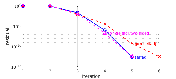
From the residual output, we can guess that the convergence is cubic (it is actually too fast to verify).
res
res =
   0.998606307083000
   0.840368825552523
   0.021040776167709
   0.000001071845020
   0.000000000000286
4. Non-selfadjoint linear operator
Now consider the non-selfadjoint operator $Au = -u'' + u' + u$, again with zero Dirichlet boundary conditions:
dom = [-pi/2, pi/2];
x = chebfun('x',dom);
A = chebop(@(x,u) -diff(u,2) + diff(u) + u, dom, 0);
I = eye(A);

% Initial guesses:
disp('lam:')
lam = 1; disp(lam)
u = randnfun(.1, dom); u = u/norm(u);
res2 = norm(A*u-lam*u)/norm(A*u);             % initial residual

% Rayleigh quotient iteration:
while ( res2(end) > tol)
    u = (A-lam*I)\u; u = u/norm(u);           % core RQI
    lam = u'*A*u; disp(lam)                   % update Rayleigh quotient
    res2 = [res2; norm(A*u-lam*u)/norm(A*u)]; % store residual
end
lam:
     1
   2.148562930010536
   2.238352474116561
   2.249952642119727
   2.249999999241508
   2.249999999999996
From the residual output, we can see that here the convergence is quadratic:
res2
res2 =
   0.999611595070082
   0.958331443919403
   0.008897560979291
   0.000035578580177
   0.000000000575788
   0.000000000000334
As before, let's try to improve the convergence to cubic. This involves the adjoint, which plays the role of the conjugate transpose in the matrix case.
% Initial guesses:
disp('lam:')
lam = 1; disp(lam)
u = randnfun(.1, dom); u = u/norm(u);         % random guess for right eigfunc
v = randnfun(.1, dom); v = v/norm(v);         % random guess for left eigfunc
res3 = norm(A*u-lam*u) / norm(A*u);

% Rayleigh quotient iteration:
while ( res3(end) > tol)
    u = (A -lam*I)\u; u = u/norm(u);          % core RQI
    v = (A'-lam*I)\v; v = v/norm(v);          % adjoint RQI
    lam = v'*(A*u)/(v'*u); disp(lam)          % update Rayleigh quotient
    res3 = [res3; norm(A*u-lam*u)/norm(A*u)]; % store residual
end

res3
lam:
     1
   2.366600934214430
   2.250150291437780
   2.249999999999692
   2.249999999999999
res3 =
   0.999549699255866
   0.980162497602524
   0.012462711448505
   0.000000200009708
   0.000000000000352
RQI appears to have computed eigenpairs for both operators, selfadjoint and non-selfadjoint. Now let's examine the convergence rates by plotting the residual convergence.
semilogy(res, 'b-o'), hold on
text(length(res) + .1, res(end), 'selfadj', 'color', 'b')
semilogy(res2, 'r--x' )
text(length(res2) - .9, res2(end-1), 'non-selfadj', 'color', 'r')
semilogy(res3, 'm--^' )
text(length(res3) - .9, res3(end-1), 'non-selfadj two-sided', 'color', 'm')
xlabel('iteration'), ylabel('residual')
grid on
5. References
- B. N. Parlett, The Symmetric Eigenvalue Problem, SIAM, 1996.