Here is a simple linear ODE boundary value problem:
$$ {dF\over dx} + 2xF = 1, \qquad F(0) = 0. $$
Chebfun can crack this problem in a few lines. Instead of a boundary condition, we will specify an interior point condition.
function DawsonIntegral
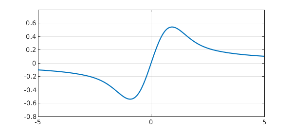
tic
W = 5; H = 0.8;
L = chebop(-W,W);
L.op = @(x,f) diff(f,1) + 2*x*f;    % ODE
L.bc = @(x,f) f(0);                 % interior point condition
f = L\1;
toc
plot(f), axis([-W W -H H]), hold on, grid on
Elapsed time is 1.066179 seconds.
The problem can be solved analytically:
$$ F(x) = e^{-x^2} \int_0^x e^{t^2} dt. $$
Users with access to the MATLAB Symbolic Toolbox could also solve it with the following code:
y = sym('y');
f(y) = sym('f(y)');
f = dsolve(diff(f) + 2*y*f == 1, f(0) == 0);
pretty(f);
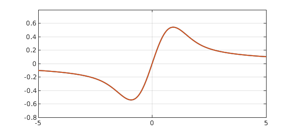
Equation (2) is known as Dawson's integral or Dawson's function, featuring a dipole structure about the origin. With the Symbolic Toolbox, you could plot the exact solution like this:
fexact = chebfun(@(x) mfun('dawson', x), [-W W]);
plot(fexact, '-.r'), hold off
On my machine, running the last few lines takes about 0.13 seconds.
It's tempting to evaluate Dawson's integral directly using Chebfun.
tic
x = chebfun('x',[0,W]);
fr = exp(-x^2)*cumsum(exp(x^2));     % right of x=0
fl = newDomain(-flipud(fr),[-W 0]);  % left of x=0
f = join(fl,fr);                     % must be an easier way to do this!
f = merge(f)
plot(f), grid on
f =
   chebfun column (2 smooth pieces)
       interval       length     endpoint values
[      -5,       0]       87      -0.1  6.2e-07
[       0,       5]       87  -6.2e-07      0.1
vertical scale = 0.54    Total length = 174
How big is the discrepancy between $F$ and $f$? You can find out by running these three lines:
semilogy(abs(f-fexact));
title('error when we evaluate F directly');
grid on, hold off
If you do, you'll find that the accuracy is only about 5 digits. It's not difficult to understand the low accuracy if we notice that Dawson's integral as shown in Equation (2) is a product of type $0 \cdot \infty$ as $x$ diverges away from the origin. A standard way to compute Dawson's integral is given in Numerical Recipes [1], where the integral is evaluated using its Maclaurin series [2,3] near the origin and Rybicki's exponentially accurate approximation [4] otherwise. It's likely that MATLAB's built-in routine adopts this algorithm.
An elegant way to evaluate Dawson's integral as well as several others in the complex error function family has been proposed by Weideman [5]. Here we borrow Weideman's eight-line MATLAB code (very slightly modified) to calculate the integral.
N = 36;
tic
f = chebfun(@(x) real(sqrt(pi)*(cef(x,N)-exp(-x^2))/2i), [-W W]);
toc
Elapsed time is 0.057716 seconds.
If you have the Symbolic Toolbox...
semilogy(abs(f-fexact)), grid on
function w = cef(z,N)      % Weideman's complex error function routine
  M = 2*N;  M2 = 2*M;  k = (-M+1:1:M-1)';      % M2 = no. of sampling points.
  L = sqrt(N/sqrt(2));                         % Optimal choice of L.
  theta = k*pi/M; t = L*tan(theta/2);          % Define variables theta and t.
  f = exp(-t.^2).*(L^2+t.^2); f = [0; f];      % Function to be transformed.
  a = real(fft(fftshift(f)))/M2;               % Coefficients of transform.
  a = flipud(a(2:N+1));                        % Reorder coefficients.
  Z = (L+1i*z)./(L-1i*z); p = polyval(a,Z);    % Polynomial evaluation.
  w = 2*p./(L-1i*z).^2+(1/sqrt(pi))./(L-1i*z); % Evaluate w(z).
end
Weideman's algorithm takes advantage of a slick rational expansion which approximates the Faddeeva function
$$ w(x) = e^{-x^2}+\frac{2i}{\sqrt{\pi}}e^{-x^2}\int_0^x e^{t^2} dt $$
uniformly accurately in the complex plane with only a small number of terms (denoted by $N$ in the code above). With $N = 36$, Dawson's integral is computed accurately within roundoff and it's done roughly ten times faster than the MATLAB Symbolic Toolbox built-in function. Amazing, isn't it? Should we suggest to MathWorks that they rewrite their Dawson function after an 18-year delay?
end
Couldn't create JOGL canvas--using painters
Couldn't create JOGL canvas--using painters
Couldn't create JOGL canvas--using painters
References
-
W. H. Press, S. A. Teukolsky, W. T. Vetterling, and B. P. Flannery, Numerical Recipes. The Art of Scientific Computing. Third edition. Cambridge University Press, Cambridge, 2007.
-
G. B. Rybicki, Dawson's integral and the sampling theorem. Computers in Physics, vol. 3 (1989), no. 2, pp. 85-87.
-
W. J. Cody, K. A. Pociorek, and H. C. Thatcher, Chebyshev approximations for Dawson's integral. Mathematics of Computation, vol. 24 (1970), pp. 171-178.
-
J. A. C. Weideman, Computation of the complex error function. SIAM Journal on Numerical Analysis, 31 (1994), no. 5, 1497-1518.