The Black-Scholes partial differential equation is the foundation of much of modern finance. Suppose you have a European-style call option (right to buy) for a certain stock, to be exercised at a time $T$ in the future. Then, as a function of the stock price $s$, the value $v(t,s)$ of the option is governed by $$ v_t = -\frac{\sigma^2}{2}s^2v_{ss} -rsv_s + rv, \quad s>0, \quad t > 0, $$ subject to $$ v(0, T) = 0, \quad v(t, s)\rightarrow s \text{ as } s\rightarrow \infty. $$
It's much more convenient for us to work on a finite domain, so we will truncate and replace the asymptotic condition with a Neumann condition.
d = [0 500];
s = chebfun('s', d);
sigma = 0.45;  r = 0.03;
A = chebop(@(s,v) -sigma^2/2*s.^2.*diff(v,2) - r*s.*diff(v) + r*v, d);
A.lbc = 0;
A.rbc = @(v) diff(v) - 1;    % replaces v->s as s->infinity
Because the PDE is linear, we can solve it using an operator exponential (i.e., $C_0$ semigroup) via expm. However, that function requires homogeneous boundary conditions, in the form $Bv=q$.
There is a very general trick to remove the nonhomoegeneous conditions, by finding a particular solution. Suppose $u(s)$ satisfies $Au=0$, $Bu=q$. Then $(v-u)_t = v_t=Av = A(v-u)$, and $B(u-v)=0$. Hence one can propagate $w=v-u$ with homogeneous conditions in combination with the solution of a boundary value problem for $u$.
u = A\0;      % u satisfies u_t = A*u = 0, B*u = q.
A.rbc = 0;    % Homogenous BCs.
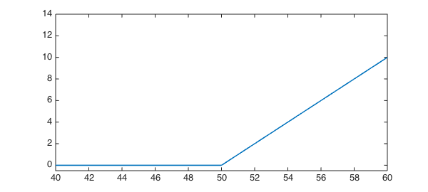
At the final time, the value of the option is the positive part of the difference between the strike price (for us, 50) and the stock price.
vT = max( 0, s-50 );
clf
plot(vT, [40 60]), hold on, ylim([-.5 14])
wT = vT - u;  % Adjusted variable - satisfies w_t = A*w, B*w = 0.
We can now evaluate at any time directly (not by marching) using the operator exponential implemented by expm. Advance in time to $t = 0.1, 0.2, ..., 0.5$ using expm:
for t = 0.1:0.1:0.5
   w = expm(A, -t, wT);
   v = w + u;
   plot(v, [40 60], 'k')
end
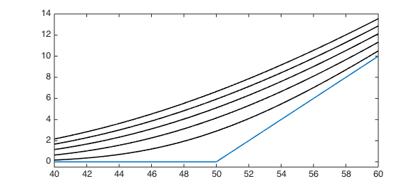
The value of this option if $s=55$, six months before the maturity date, is
v(55)
ans =
   9.849887661936435
Note that the initial condition for $w$ is piecewise defined. Thus, w will be piecewise at all times in Chebfun.
w
w =
   chebfun column (1 smooth piece)
       interval       length   endpoint values
[       0,   5e+02]       97     5e-11  7.9e-12
Epslevel = 4.510522e-13.  Vscale = 4.925018e+01.
However, the solution is actually smooth.
wss = diff(w,2);
jump2 = wss(50+100*eps) - wss(50-100*eps)
jump2 =
    -2.428612866367530e-17