KdV solitons and non-solitons

1. Soliton solutions

Chebfun's spin command [1] makes it easy to compute solutions of the KdV equation, $$ u_t = -0.5(u^2)_x - u_{xxx}. $$ For example, let's set to work on $[0,20]$ with a two-soliton initial condition $$ u_0(x) = 3A^2 \hbox{sech}(.5A(x-1))^2 + 3B^2 \hbox{sech}(.5B(x-2))^2 $$ where the amplitude parameters $A$ and $B$ are quite close to each other, taking values $25$ and $23$. We can set up for the calculation like this:

A = 25; B = 23;
dom = [0 20]; x = chebfun('x',dom);
tmax = 0.0156;
S = spinop(dom,[0 tmax]);
S.lin = @(u) - diff(u,3);
S.nonlin = @(u) -.5*diff(u.^2); % spin cannot parse "u.*diff(u)"
S.init = 3*A^2*sech(.5*A*(x-3)).^2 + 3*B^2*sech(.5*B*(x-4)).^2;

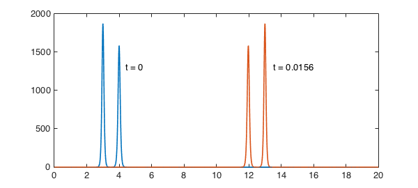
Now let's perform the calculation. This initial condition corresponds to a pair of solitons with slightly different amplitudes and different speeds. As $t$ increases, both pulses move right, with the taller one moving faster. Around time $t=0.0078$, it overtakes the slower one, and around time $t=0.0156$, it is as far ahead at was originally behind.

N = 800;   % numer of grid points
dt = 5e-6; % time-step
tic, u = spin(S,N,dt,'plot','off'); time_in_seconds = toc;
plot(S.init), hold on, plot(u), hold off
text(4.4,1300,'t = 0'), text(13.5,1300,'t = 0.0156')

With the dicretization we used, the computation is quite fast:

time_in_seconds

time_in_seconds =
   1.395754691000000

2. Amplitude and speed

Let's look at the propagation of a single soliton, the larger one from the last experiment:

S.init = 3*A^2*sech(.5*A*(x-3)).^2;
u = spin(S,N,dt,'plot','off');
plot(S.init), hold on, plot(u), hold off
text(3.4,1300,'t = 0'), text(13.2,1300,'t = 0.0156')

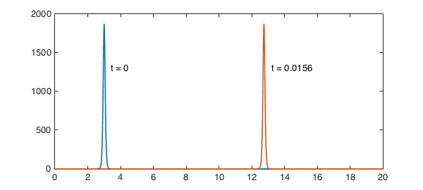
The initial amplitude is

initial_amplitude = 3*A^2

initial_amplitude =
        1875

and we see that this is the same at the end (mathematically it would be identical):

[val,pos] = max(u);
final_amplitude = val

final_amplitude =
     1.874048194434761e+03

What about the speed? According to the theory of the KdV equation, this should be

predicted_speed = A^2

predicted_speed =
   625

Here is the computed value:

observed_speed = (pos-3)/tmax

observed_speed =
     6.248377320106790e+02

3. Non-soliton solutions

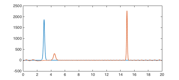
Soliton solutions are so celebrated that it is easy to forget that they are special. Let us explore various other possibilities. First of all, what if we make the initial pulse a bit wider, so that it is no longer a soliton? As $t$ increases, the wave now breaks into a big soliton travelling at about the same speed as before and a small one going much more slowly, plus some low-amplitude information that is not in the form of solitons.

S.init = 3*A^2*sech(.35*A*(x-3)).^2;
u = spin(S,N,dt,'plot','off');
plot(S.init), hold on, plot(u), hold off

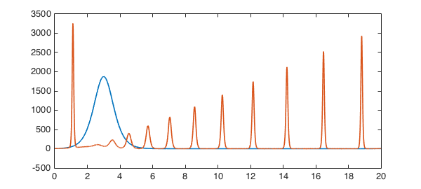
If we make the pulse still wider, we get a beautiful train of solitons. Note that a term centered at $x=23$ has been added to make this wider pulse numerically periodic.

S.init = 3*A^2*( sech(.05*A*(x-3)).^2 + sech(.05*A*(x-23)).^2 );
u = spin(S,N,dt,'plot','off');
plot(S.init), hold on, plot(u), hold off

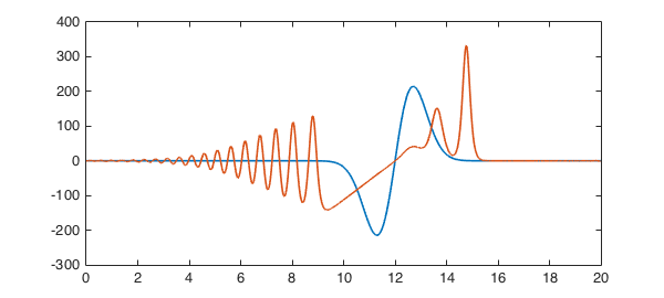
Let's try something a little bit random:

S.init = 500*(x-12).*exp(-(x-12).^2);
u = spin(S,N,dt,'plot','off');
plot(S.init), hold on, plot(u), hold off

4. Conservation laws

The function $u$ is a conserved quantity for the KdV equation in the sense that its integral remains constant. Here we confirm this numerically (the integral is zero since the function is odd):

u0 = S.init;
conserved1 = @(u) sum(u)
conserved1(u), conserved1(u0)

conserved1 = 
    @(u)sum(u)
ans =
     3.513633828333696e-13
ans =
     3.241851231905457e-13

Another conserved quantity is $u^2$:

conserved2 = @(u) sum(u.^2)
conserved2(u), conserved2(u0)

conserved2 = 
    @(u)sum(u.^2)
ans =
     7.833213357987507e+04
ans =
     7.833213358221899e+04

In fact, as a completely integrable system, the KdV equation has an infinite set of conserved quantities [3,4]. Another one is $u^3/3 - (u_x)^2$:

conserved3 = @(u) sum(u.^3/3 - diff(u).^2)
conserved3(u), conserved3(u0)

conserved3 = 
    @(u)sum(u.^3/3-diff(u).^2)
ans =
    -2.349964008126170e+05
ans =
    -2.349964007466422e+05

Another is $u^4/4 - 3u(u_x)^2 + (9/5)(u_{xx})^2$:

conserved4 = @(u) sum(u.^4/4 - 3*u.*diff(u).^2 + (9/5)*diff(u,2).^2)
conserved4(u), conserved4(u0)

conserved4 = 
    @(u)sum(u.^4/4-3*u.*diff(u).^2+(9/5)*diff(u,2).^2)
ans =
     6.512069540200268e+08
ans =
     6.512069540223168e+08

And so on in an infinite sequence.

5. References

The mathematics of solitons is thoroughly understood. See for example [2]. For a quick introduction to the KdV equation, see [3].

[1] H. Montanelli and N. Bootland, Solving periodic semilinear stiff PDEs in 1D, 2D and 3D with exponential integrators, submitted, 2016.

[2] M. J. Ablowitz and H. Segur, Solitons and the Inverse Scattering Transform, SIAM, 1981.

[3] L. N. Trefethen and K. Embree, editors, article on "The KdV equation", The (Unfinished) PDE Coffee Table Book, https://people.maths.ox.ac.uk/trefethen/pdectb.html.