function AverageDegreeReduction2D

2D subdivision

Generally, Chebfun2 approximates globally smooth functions $f(x,y)$ by global low rank polynomial interpolants. However, in the bivariate rootfinding algorithm to solve

$$ f(x,y) = g(x,y) = 0, $$

we use piecewise smooth interpolants if the polynomial degrees are larger than $16$ in the $x$- or $y$-variable (of $f$ or $g$). In bivariate rootfinder the resultant based method recursively subdivides the rectangular domain and the functions $f(x,y)$ and $g(x,y)$ are approximated by piecewise smooth bivariate polynomial interpolants with each piece of degree at most $16$. Subdivision is useful for reducing the complexity of the bivariate rootfinding algorithm. The reduction in the complexity is determined by a parameter $\tau$ that measures the average degree reduction. Essentially subdivision means that much higher degree problems can be solved (see [1,2]).

The average degree reduction parameter

The parameter $\tau$ measures the average reduction in polynomial degrees of $f(x,y)$. That is, if a polynomial of degree $n$ (in the $x$- and $y$-variable) is required to approximate $f(x,y)$ on $[-1,1]\times[-1,1]$ then the average degree required to approximate $f$ on $[-1,r]\times[-1,s]$ (and the other subdomains) is $\tau n$, where $r$ and $s$ are two small arbitrary constants. Throughout this Example we take symmetric functions, i.e., $f(x,y) = f(y,x)$ since then the degree reduction is identical in the $x$ and $y$ direction, which considerably simplifies the discussion. The average degree reduction parameter was introduced in [1].

Rank one functions

A function $f(x,y)$ is of rank $1$ if it can can be written as a product of univariate functions, i.e., $f(x,y) = h(x)k(y)$. Since in this example we are considering only symmetric functions we have $f(x,y) = h(x)h(y)$. For rank $1$ functions the average degree reduction parameter is typically about $1/2$ because under subdivision the degree reduction is directly determined by the degree reduction in $h(x)$. The average degree reduction parameter for univariate functions is discussed in [2]. For example,

M = 2000;
f = @(x,y) sin(M*x).*sin(M*y);
compute_tau(f, 2)          % Expected to be approximately 1/2

Tau = 0.33178

The parameter $\tau$ in this case is equal to $1/2$ because the number of oscillations of $f(x,y)$ in a rectangular domain $[a,b]\times[c,d]$ is directly proportional to $(b-a)(d-c)$. Moreover, the number of oscillations determines the number of points required to resolve the function. Therefore, each subdivision (in the $x$ or $y$ direction) halves the numerical degree of the polynomial interpolant and $\tau \approx 1/2$.

Here is a diagram that shows the numerical degrees after each level of subdivision:

subdivisionDiagram(f)

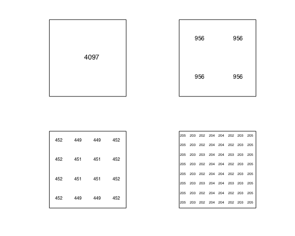
In general, if $h(x)$ is a univariate function with average degree reduction parameter $\tau$ then the rank $1$ function $f(x,y) = h(x)h(y)$ has the same average degree reduction parameter.

Toeplitz functions

A function $f(x,y)$ on $[-1,1]\times[-1,1]$ is defined as Toeplitz if there is a univariate function $h(t)$ on $[-2,2]$ such that $f(x,y) = h(x-y)$. Functions in this class are typically of rank at least two and the average degree reduction parameter cannot be understood from the univariate setting.

M = 20;
f = @(x,y) sin(M*(x-y));
compute_tau(f, 2)          % Expected to be approximately 1/sqrt(2) = 0.707

Tau = 1.30609

The average $\tau$ parameter can be explained since all the oscillations of $f$ occur along diagonals, i.e., $y=-x$ (rather than in the coordinate directions). Two subdivisions, one in the $x$ and one in the $y$ direction are required to halve the length of the diagonal lines and hence, $\tau^2 \approx 1/2$ and $\tau = 1/\sqrt{2}$.

Here is a diagram that shows the numerical degrees after each level of subdivision:

clf, subdivisionDiagram(f)

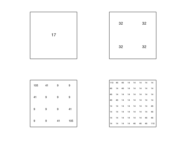
It can be seen that the numerical degree reduces by a factor of approximately $1/\sqrt{2}$ on each subdivision:

[m,n]=length(chebfun2(f));
max(m,n)./2.^(0:.5:1.5)

ans =
  Columns 1 through 3
  65.000000000000000  45.961940777125584  32.500000000000000
  Column 4
  22.980970388562795

Symmetric Cauchy function

The symmetric Cauchy function is given by $f(x,y) = 1/(x+y)$ defined on $[a,b]\times[a,b]$, where $0<a<b$. This is a 2D generalisation of functions of the form $1/(x+c)$, which has been used to investigate the parameter $\tau$ in the univariate case [2]. The numerical degree of $f(x,y)$ can be determined by using Eliott's method for all $0<a<b$.

However, this is an example where the average degree reduction depends on the subdivision level. Initially subdivision is very helpful, but as more levels are taken subdivision helps less. For example,

a = 1; b = 100;
f = @(x,y) 1./((b-a)/2*((x+1)+(y+1))+2*a);  %f = 1/(x+y) on [a,b]x[a,b]
clf, subdivisionDiagram(f)

Using Elliott's method we have an exact formula for the numerical degree of $f$, for example, the numerical degree in the bottom-left subdomain should be the following:

j=1;
for b = [100 50 25 17.5]
    a = 1; r = b/a;
    B = (r+3)/(r-1);
    m(j) = ceil(log(4/(r-1)*eps^(-1)/sqrt(B^2-1))/log(B+sqrt(B^2-1)));
    j=j+1;
end
m.'

ans =
   121
    86
    62
    52

Conclusion

Subdivision is an important technique for rootfinding to reduce the complexity of a rootfinding algorithm. Subdivision is most effective when the average degree reduction parameter is small (such as for rank one functions). Typically, we observe the $\tau$ parameter is approximately $1/\sqrt{2} = 0.707$ for bivariate functions.

function compute_tau(f, N)
% COMPUTE_TAU estimate the average degree reduction parameter
g = chebfun2(f); tol = 1e-14;
X = chebcoeffs2(g);
L = find(max(abs(rot90(X,2))) < tol,1,'last');
x = linspace(-1,1,2.^N+1);
tot = 0;
%[xx,yy] = meshgrid(x);
for j = 1:length(x)-1
    for k = 1:length(x)-1
        g = chebfun2(f, [x(j:j+1) x(k:k+1)]);
        X = chebcoeffs2(g);
        len = find(max(abs(rot90(X,2))) < tol,1,'last');
        tot = tot + len;
    end
end
avg = tot./(length(x)-1).^2;
tau = (avg/L).^(1./N);
fprintf('Tau = %1.5f',tau);
end

function subdivisionDiagram(f)
% SUBDIVISIONDIAGRAM draw a diagram to show subdivision and polynomial
% degrees.
LW = 'linewidth'; lw = 1;
FS = 'fontsize';
tol = 1e-14;
set(gcf, 'position', [0 0 600 480]), hold on
for levels = 0:3
    fs = round(14-2.5*levels);
    subplot(2,2,levels+1)
    x = linspace(-1,1,2.^levels+1);
    if levels > 0
        plot([-1,1],[x;x].','k-',LW,lw),
        plot([x;x].',[-1,1],'k-',LW,lw), axis equal
    end
    plot([-1 1 1 -1 -1],[-1 -1 1 1 -1],'k-',LW,lw), axis equal
    for j = 1:length(x)-1
        for k = 1:length(x)-1
            g = chebfun2(f, [x(j:j+1) x(k:k+1)]);
            X = chebcoeffs2(g);
            len = find(max(abs(rot90(X,2))) < tol,1,'last');
            text(mean(x(j:j+1))-.1,mean(x(k:k+1)),sprintf('%u',len),FS,fs)
        end
    end
    axis(1.05*[-1,1,-1,1]), axis off
end
end

end

References

1. Y. Nakatsukasa, V. Noferini, and A. Townsend, Computing the common zeros of two bivariate functions via Bezout resultants, Numerische Mathematik, to appear.

2. A. Townsend, 1D Subdivision and the average degree reduction, Chebfun Example, May 2013.

3. A. Townsend and L. N. Trefethen, An extension of Chebfun to two dimensions, SIAM Journal on Scientific Computing, 35 (2013), C495-C518.