My essay "Six myths of polynomial interpolation and quadrature", reproduced as an appendix in [1], closes with an example that reminds one of a tiger's tail. Here with a few modifications is that example:

x = chebfun('x',[-2 1]);
CO = 'color'; orange = [1 .5 .25];
f = 2*exp(.5*x).*(sin(5*x) + sin(101*x));
roundf = round(f);
r = roots(f-roundf,'nojump');
hold off, plot(f,CO,orange), hold on
ylim([-8 6])
plot(r,f(r),'.k'), hold off

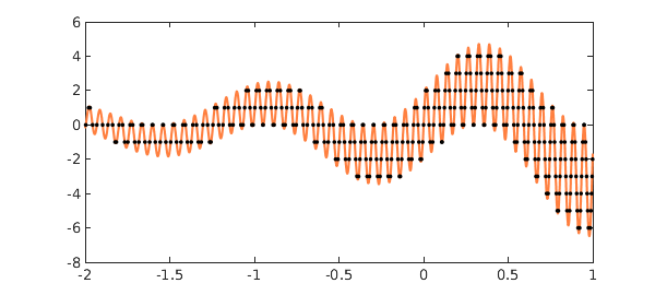
Let's look at what's going on here. First of all a chebfun $f$ is constructed:

plot(f,CO,orange)
ylim([-8 6])

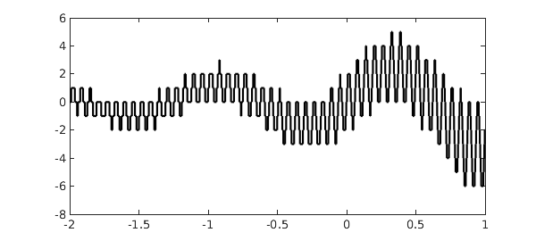
Then another chebfun is constructed consisting of $f$ rounded to integers:

plot(roundf,'k','jumpline','k')
ylim([-8 6])

Superimposing the two curves yields a lot of intersections, which are computed by roots:

number_of_roots = length(r)
plot(f,CO,orange), hold on
plot(roundf,'k','jumpline','k')
plot(r,f(r),'.k'), hold off

number_of_roots =
   345

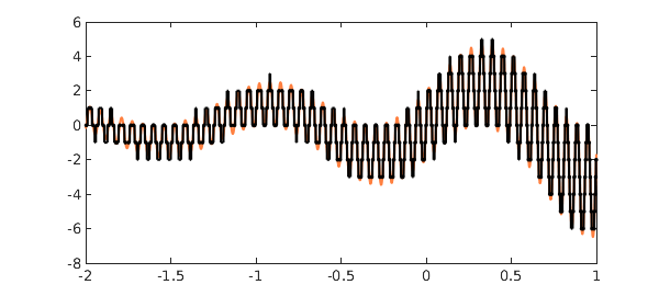
In [1], dots appear not only where $f$ is equal to an integer, but also where it is equal to a half-integer. In the present version of the tiger's tail, this effect has been eliminated by use of the 'nojump' flag in roots.

Reference

1. L. N. Trefethen, Approximation Theory and Approximation Practice, Extended Edition, SIAM, 2019.