1. Introduction

Probability and statistics textbooks contain many exercise problems concerning various probability distributions. In this Example we use Chebfun to solve a problem involving the normal distribution from the textbook [1]. Other similar Examples look at problems from the same book involving the exponential, beta, gamma, Rayleigh, and Maxwell distributions.

Like most textbooks, [1] emphasizes problems that can be solved on paper and don't need numerical tools such as Chebfun. As soon as one varies the problem a little, however, numerical solutions often become necessary. Thus first we solve the problem as written, and then we solve a variant.

2. Problem 1(d), page 124

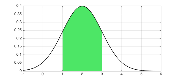
If $X$ is normally distributed with mean $2$ and variance $1$, find $P[|X-2|<1]$.

The probability density function (PDF) of the normal distribution can be defined like this:

ff = @(x,mu,sigma) 1/(sigma*sqrt(2*pi))*exp(-0.5*((x-mu)/sigma).^2);

The domain is the entire real line, and this is a case where Chebfun has no difficulty working with that domain. We can construct the chebfun like this:

mu = 2;
sigma = 1;
f = chebfun(@(x) ff(x,mu,sigma), [-inf,inf]);

The cumulative density function (CDF) is the indefinite integral of $f$:

fint = cumsum(f);

We can find the probability of $P[|X-2|<1]$ like this:

format long
p = fint(3)-fint(1)

p =
   0.682689492136379

Let's plot $f$ and the region $|X-2|<1$:

hold off, h = area(f{1,3});
set(h,'FaceColor',[0.3 0.9 0.4]), axis auto
LW = 'linewidth';
hold on, plot(f,'k',LW,1.6,'interval',[-1 6]), grid on

3. Problem 1(d), page 124 -- numerical variant

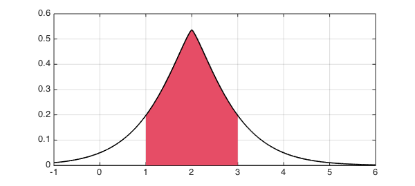
Now let us do a similar computation, except replacing the quadratic term in the normal distribution by an absolute value with a $5/4$ power.

ff = @(x,mu,sigma) exp(-abs((x-mu)/sigma).^(5/4));

The factor $1/\sqrt{2\pi\sigma}$ has been deleted because now we will have to normalize the distribution by hand. Here is the normalized chebfun:

f = chebfun(@(x) ff(x,mu,sigma), [-inf,inf],'splitting','on');
f = f/sum(f);

We can compute the probability as before:

fint = cumsum(f);
p = fint(3)-fint(1)

p =
   0.718570707764524

And here is a plot, with a new color for variety:

hold off, h = area(f{1,3});
set(h,'FaceColor',[0.9 0.3 0.4]), axis auto
hold on, plot(f,'k',LW,1.6,'interval',[-1 6]), grid on

References

1. A. M. Mood, F. A. Graybill, and D. Boes, Introduction to the Theory of Statistics, McGraw-Hill, 1974.