Numerical computing with functions

Chebfun is an open-source package for computing with functions to about 15-digit accuracy. Most Chebfun commands are overloads of familiar MATLAB commands — for example sum(f) computes an integral, roots(f) finds zeros, and u = L\f solves a differential equation.

DOWNLOAD V5.7.0BROWSE SOURCE

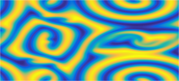
% Create operator for Ginzburg-Landau problem
d = 20*[-1.2 3.2 -1 1];  tspan = [0 46.5];
S = spinop2(d,tspan); S.lin = @(u) lap(u);
S.nonlin = @(u) u - (1+1.5i)*u.*(abs(u).^2);
% Set initial condition, solve PDE, plot
S.init = chebfun2(@(x,y) ...
    (1i*x+y).*exp(-.03*(x.^2+y.^2)), d);
u = spin2(S, 128, 1e-1, 'plot', 'off');
plot(real(u))

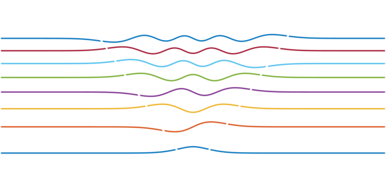
% Create a chebfun on the interval [-3,3]
x = chebfun('x', [-3 3]);
% Define a potential function
V = abs(x);
% Plot the first 8 eigenstates of
% the Schrodinger operator
quantumstates(V, 8)

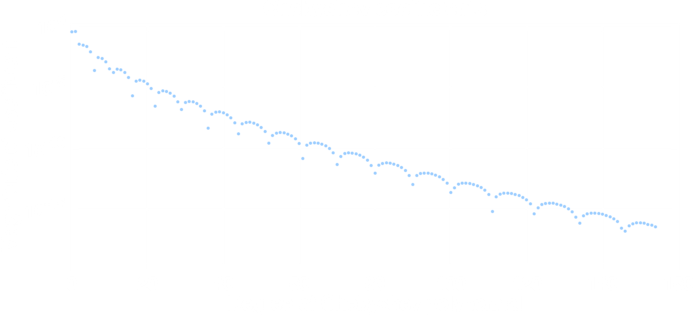
% Create a chebfun f
x = chebfun('x');
f = exp(-1./(x+1));
% Plot abs vals of Chebyshev coeffs of f
plotcoeffs(f,'.')

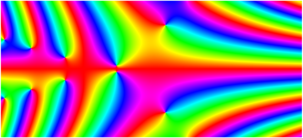
% Define a rectangular domain
d = pi*[-2.2 2.2 -1 1]/2;
% Create a complex-valued chebfun2
f = chebfun2(@(z) ...
    cos((z-1).^2)+exp((z+1).^2), d);
% Plot its phase portrait
plot(f)

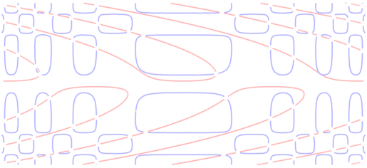
% Construct a pair of 2D chebfuns
d = [-3 10 -3 3];
f = chebfun2('y.*cos(y.^2+x)-.1',d);
g = chebfun2('cos(x.^2/2).*sin(y.^2)-.1',d);
% Plot zero contours of f & g
plot(roots(f)), hold on, plot(roots(g))
% Plot their common roots
r = roots(f, g, 'resultant');
plot(r(:,1), r(:,2), '.')

% Define two functions
f = chebfun(@(x) sin(x.^2)+sin(x).^2, [0,10]);
g = chebfun(@(x) exp(-(x-5).^2/10), [0,10]);
% Compute their intersections
rr = roots(f - g);
% Plot the functions
plot([f g]), hold on
% Plot the intersections
plot(rr, f(rr), 'o')

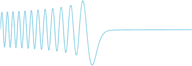
% Airy operator
op = @(x,u) 0.01*diff(u,2) - x.*u;
% Create a chebop
L = chebop(op, [-5,5]);
% Apply boundary conditions
L.bc = 'dirichlet';
% Solve the differential equation
u = L \ 1;
plot(u)

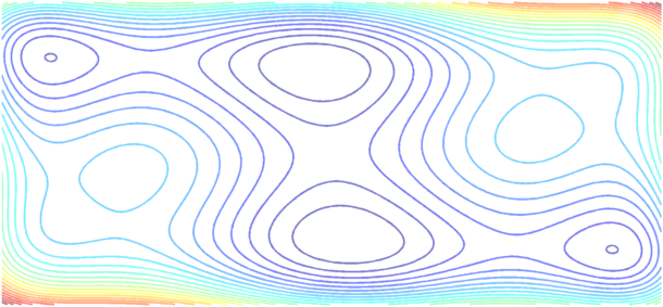
% The Dixon-Szego function
f = @(x,y) (4-2.1*x.^2+ x.^4/3).*x.^2 ...
            + x.*y + 4*(y.^2-1).*y.^2;
% Create a chebfun2
F = chebfun2(f, [-2,2,-1.25,1.25]);
% Find the minimum and mark it
[minf,minx] = min2(F);
contour(F,30), hold on
plot(minx(1),minx(2),'.w')

Check out the Chebfun users group!

Chebfun—numerical computing with functions

Latest news

10 June 2018/Default GitHub branch switched from development to master

9 January 2018/One-week course at ENS-Lyon by Nick Trefethen

Download »

Get started »

View Examples »