2.1 sum
We have seen that sum returns the definite integral of a chebfun over its range of definition. The integral is normally calculated by an FFT-based version of Clenshaw-Curtis quadrature, as described first in [Gentleman 1972]. This formula is applied on each fun (i.e., each smooth piece of the chebfun), and then the results are added up.
Here is an example whose answer is known exactly:
  f = chebfun(@(x) log(1+tan(x)),[0 pi/4]);
  format long
  I = sum(f)
  Iexact = pi*log(2)/8
I =
   0.272198261287950
Iexact =
   0.272198261287950
Here is an example whose answer is not known exactly, given as the first example in the section "Numerical Mathematics in Mathematica" in The Mathematica Book [Wolfram 2003].
  f = chebfun('sin(sin(x))',[0 1]);
  sum(f)
ans =
   0.430606103120691
All these digits match the result $0.4306061031206906049\dots$ reported by Mathematica.
Here is another example:
  F = @(t) 2*exp(-t.^2)/sqrt(pi);
  f = chebfun(F,[0,1]);
  I = sum(f)
I =
   0.842700792949715
The reader may recognize this as the integral that defines the error function evaluated at $t=1$:
Iexact = erf(1)
Iexact =
   0.842700792949715
It is interesting to compare the times involved in evaluating this number in various ways. MATLAB's specialized erf code is the fastest:
tic, erf(1), toc
ans =
   0.842700792949715
Elapsed time is 0.000158 seconds.
Using MATLAB's quadrature command is understandably slower:
  tol = 3e-14;
  tic, I = integral(F,0,1,'abstol',tol,'reltol',tol); t = toc;
    fprintf(' MATLAB:  I = %17.15f  time = %6.4f secs\n',I,t)
MATLAB: I = 0.842700792949715 time = 0.0351 secs
The timing for Chebfun comes out competitive:
  tic, I = sum(chebfun(F,[0,1])); t = toc;
    fprintf('CHEBFUN:  I = %17.15f  time = %6.4f secs\n',I,t)
CHEBFUN: I = 0.842700792949715 time = 0.0098 secs
(Chebfun also offers an integral command, which is just a wrapper that calls sum as above.)
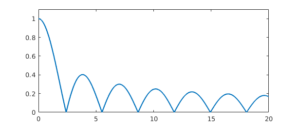
Here is a similar comparison for a function that is more difficult, because of the absolute value, which leads with "splitting on" to a chebfun consisting of a number of funs.
  F = @(x) abs(besselj(0,x));
  f = chebfun(@(x) abs(besselj(0,x)),[0 20],'splitting','on');
  plot(f), ylim([0 1.1])
  tol = 3e-14;
  tic, I = integral(F,0,20,'abstol',tol,'reltol',tol); t = toc;
    fprintf(' MATLAB:  I = %17.15f  time = %5.3f secs\n',I,t)
  tic, I = sum(chebfun(@(x) abs(besselj(0,x)),[0,20],'splitting','on')); t = toc;
    fprintf('CHEBFUN:  I = %17.15f  time = %5.3f secs\n',I,t)
 MATLAB:  I = 4.445031603001577  time = 0.018 secs
CHEBFUN:  I = 4.445031603001566  time = 0.065 secs
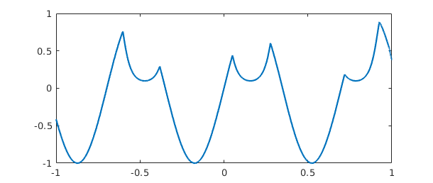
This last example highlights the piecewise-smooth aspect of Chebfun integration. Here is another example of a piecewise smooth problem.
  x = chebfun('x');
  f = sech(3*sin(10*x));
  g = sin(9*x);
  h = min(f,g);
  plot(h)
Here is the integral:
tic, sum(h), toc
ans =
  -0.381556448850250
Elapsed time is 0.001830 seconds.
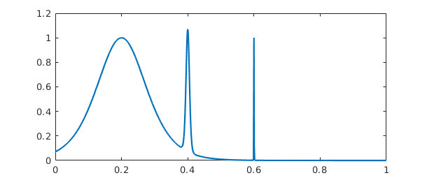
For another example of a definite integral we turn to an integrand given as example F21F in [Kahaner 1971] (see also cheb.gallery('kahaner')). We treat it first in the default mode of splitting off:
  ff = @(x) sech(10*(x-0.2))^2 + sech(100*(x-0.4))^4 + ...
            sech(1000*(x-0.6))^6;
  f = chebfun(ff,[0,1])
f =
   chebfun column (1 smooth piece)
       interval       length     endpoint values
[       0,       1]    14036     0.071  4.5e-07
vertical scale = 1.1
The function has three spikes, each ten times narrower than the last:
plot(f)
The length of the global polynomial representation is accordingly quite large, but the integral comes out correct to full precision:
  length(f)
  sum(f)
ans =
       14036
ans =
   0.210802735500549
With splitting on, Chebfun also gets the right answer, and note that the length of the chebfun is much smaller than before:
  f = chebfun(ff,[0,1],'splitting','on');
  length(f)
  sum(f)
ans =
   399
ans =
   0.210802735500549
Earlier versions of Chebfun used to get this wrong, in which case the problem could be fixed by forcing finer initial sampling in the Chebfun constructor with the minSamples flag. For more about minSamples, see Section 8.6.
  f = chebfun(ff,[0,1],'splitting','on','minSamples',100);
  length(f)
  sum(f)
ans =
   399
ans =
   0.210802735500549
As mentioned in Chapter 1 and described in more detail in Chapter 9, Chebfun has some capability of dealing with functions that blow up to infinity. Here for example is a familiar integral:
  f = chebfun(@(x) 1/sqrt(x),[0 1],'blowup',2);
  sum(f)
ans =
   2.000000000000000
Certain integrals over infinite domains can also be computed, though the error is often large:
  f = chebfun(@(x) 1/x^2.5,[1 inf]);
  sum(f)
Warning: Result may not be accurate as the function decays slowly at infinity.
ans =
   0.666666667492359
Chebfun is not a specialized item of quadrature software; it is a general system for manipulating functions in which quadrature is just one of many capabilities. Nevertheless Chebfun compares reasonably well as a quadrature engine against specialized software. This was the conclusion of an Oxford MSc thesis by Phil Assheton [Assheton 2008], which compared Chebfun experimentally to quadrature codes available at that time including MATLAB's quad and quadl, Gander and Gautschi's adaptsim and adaptlob, Espelid's modsim, modlob, coteda, and coteglob, QUADPACK's QAG and QAGS, and the NAG Library's d01ah. In both reliability and speed, Chebfun was found to be competitive with these alternatives. The overall winner was coteda [Espelid 2003], which was typically about twice as fast as Chebfun. For further comparisons of quadrature codes, together with the development of some improved codes based on a philosophy that has something in common with Chebfun, see [Gonnet 2009]. See also "Battery test of Chebfun as an integrator" in the Quadrature section of the Chebfun Examples collection.
2.2 norm, mean, std, var
A special case of an integral is the norm command, which for a chebfun returns by default the 2-norm, i.e., the square root of the integral of the square of the absolute value over the region of definition. Here is a well-known example:
norm(chebfun('sin(pi*theta)'))
ans =
     1
If we take the sign of the sine, the norm increases to $\sqrt 2$:
norm(chebfun('sign(sin(pi*theta))','splitting','on'))
ans =
   1.414213562373095
Here is a function that is infinitely differentiable but not analytic.
  f = chebfun('exp(-1/sin(10*x)^2)');
  plot(f)
Here are the norms of f and its tenth power:
norm(f), norm(f^10)
ans =
   0.292873834331035
ans =
     2.187941295308668e-05
2.3 cumsum
In MATLAB, cumsum gives the cumulative sum of a vector,
  v = [1 2 3 5]
  cumsum(v)
v =
     1     2     3     5
ans =
     1     3     6    11
The continuous analogue of this operation is indefinite integration. If f is a fun of length $n$, then cumsum(f) is a fun of length $n+1$ or less (because of Chebfun's rounding of functions to machine precision). For a chebfun consisting of several funs, the integration is performed on each piece.
For example, returning to an integral computed above, we can make our own error function like this:
  t = chebfun('t',[-5 5]);
  f = 2*exp(-t^2)/sqrt(pi);
  fint = cumsum(f);
  plot(fint,'m')
  ylim([-0.2 2.2]), grid on
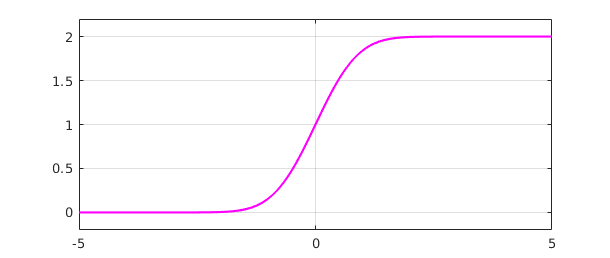
The default indefinite integral takes the value $0$ at the left endpoint, but in this case we would like $0$ to appear at $t=0$:
  fint = fint - fint(0);
  plot(fint,'m')
  ylim([-1.2 1.2]), grid on

The agreement with the built-in error function is convincing:
[fint((1:5)') erf((1:5)')]
ans =
   0.842700792949715   0.842700792949715
   0.995322265018953   0.995322265018953
   0.999977909503001   0.999977909503001
   0.999999984582742   0.999999984582742
   0.999999999998463   0.999999999998463
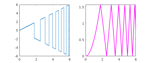
Here is the integral of an oscillatory step function:
  x = chebfun('x',[0 6]);
  f = x*sign(sin(x^2)); subplot(1,2,1), plot(f)
  g = cumsum(f); subplot(1,2,2), plot(g,'m')
And here is an example from number theory. The logarithmic integral, $Li(x)$, is the indefinite integral from $0$ to $x$ of $1/\log(s)$. It is an approximation to $\pi(x)$, the number of primes less than or equal to $x$. To avoid the singularity at $x=0$ we begin our integral at the point $\mu = 1.451...$ where $Li(x)$ is zero, known as Soldner's constant. The test value $Li(2)$ is correct except in the last few digits:
  mu = 1.45136923488338105;      % Soldner's constant
  xmax = 400;
  Li = cumsum(chebfun(@(x) 1/log(x),[mu xmax]));
  lengthLi = length(Li)
  Li2 = Li(2)
lengthLi =
   411
Li2 =
   1.045163780117470
(Chebfun has no trouble if xmax is increased to $10^5$ or $10^{10}$.) Here is a plot comparing $Li(x)$ with $\pi(x)$:
  clf, plot(Li,'m')
  p = primes(xmax);
  hold on, plot(p,1:length(p),'.k'), hold off
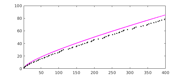
The Prime Number Theorem implies that $\pi(x) \sim Li(x)$ as $x\to\infty$. Littlewood proved in 1914 that although $Li(x)$ is greater than $\pi(x)$ at first, the two curves eventually cross each other infinitely often. It is known that the first crossing occurs somewhere between $x=10^{14}$ and $x=2\times 10^{316}$ [Kotnik 2008].
The mean, std, and var commands have also been overloaded for chebfuns and are based on integrals. For example,
mean(chebfun('cos(x)^2',[0,10*pi]))
ans =
   0.500000000000000
2.4 diff
In MATLAB, diff gives finite differences of a vector:
  v = [1 2 3 5]
  diff(v)
v =
     1     2     3     5
ans =
     1     1     2
The continuous analogue of this operation is differentiation. For example:
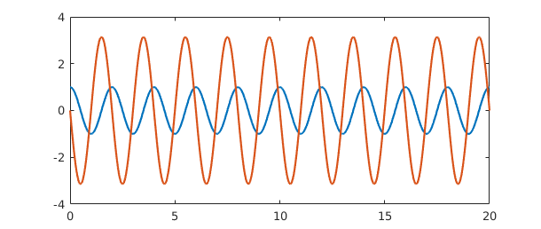
  f = chebfun('cos(pi*x)',[0 20]);
  fprime = diff(f);
  plot([f fprime])
If the derivative of a function with a jump is computed, then a delta function is introduced. Consider for example this function defined piecewise:
  f = chebfun({@(x) x^2, 1, @(x) 4-x, @(x) 4/x},0:4);
  plot(f)
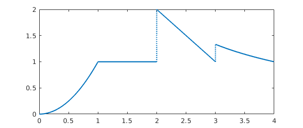
Here is the derivative:
  fprime = diff(f);
  plot(fprime,'r'), ylim([-2,3])
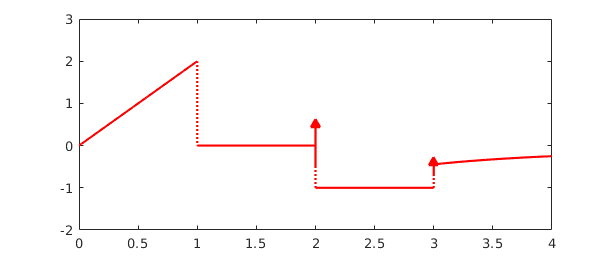
The first segment of $f'$ is linear, since $f$ is quadratic here. Then comes a segment with $f' = 0$, since $f$ is constant. At the end of this second segment appears a delta function of amplitude $1$, corresponding to the jump of $f$ by $1$. The third segment has constant value $f' = -1$. Finally another delta function, this time with amplitude $1/3$, takes us to the final segment.
Thanks to the delta functions, cumsum and diff are essentially inverse operations. It is no surprise that differentiating an indefinite integral returns us to the original function:
norm(f-diff(cumsum(f)))
ans =
     2.250689041652248e-16
More surprising is that integrating a derivative does the same, as long as we add in the value at the left endpoint:
  d = domain(f);
  f2 = f(d(1)) + cumsum(diff(f));
  norm(f-f2)
ans =
     2.220446049250313e-16
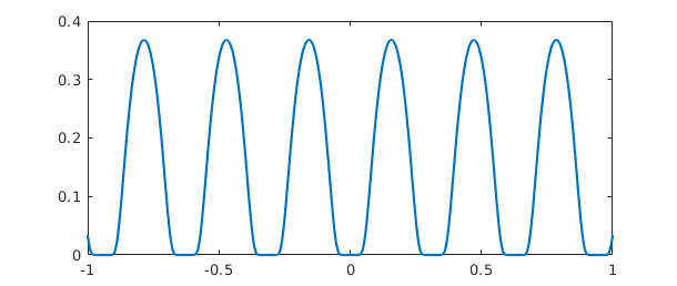
Multiple derivatives can be obtained by adding a second argument to diff. Thus for example,
  f = chebfun('1/(1+x^2)');
  g = diff(f,4); plot(g)
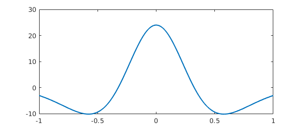
However, one should be cautious about the potential loss of information in repeated differentiation of nonperiodic chebfuns. For example, if we evaluate this fourth derivative at $x=0$ we get an answer that matches the correct value $24$ only to $11$ places:
g(0)
ans =
  24.000000000068720
For a more extreme example, suppose we define a chebfun for $\exp(x)$ on $[-1,1]$:
  f = chebfun('exp(x)');
  length(f)
ans =
    15
Differentiation is a notoriously ill-posed problem, and since $f$ is a polynomial of low degree, it cannot help but lose information rather fast as we differentiate. In fact, differentiating $15$ times eliminates the function entirely.
  for j = 0:length(f)
    fprintf('%6d %19.12f\n', j,f(1))
    f = diff(f);
  end
     0      2.718281828459
     1      2.718281828459
     2      2.718281828458
     3      2.718281828438
     4      2.718281827790
     5      2.718281811104
     6      2.718281472937
     7      2.718276094326
     8      2.718208457459
     9      2.717533872966
    10      2.712224747871
    11      2.679770038301
    12      2.530374129594
    13      2.041046024647
    14      1.020835497184
    15      0.000000000000
Is such behavior "wrong"? Well, that is an interesting question. Chebfun is behaving correctly in the sense mentioned in the second paragraph of Section 1.1: the operations are individually stable in that each differentiation returns the exact derivative of a function very close to the right one. The trouble is that because of the intrinsically ill-posed nature of differentiation, the errors in these stable operations accumulate exponentially as successive derivatives are taken.
2.5 Integrals in two dimensions
Chebfun can often do a pretty good job with integrals over rectangles. Here for example is a colorful function:
  r = @(x,y) sqrt(x.^2+y.^2); theta = @(x,y) atan2(y,x);
  f = @(x,y) sin(5*(theta(x,y)-r(x,y))).*sin(x);
  x = -2:.02:2; y = 0.5:.02:2.5; [xx,yy] = meshgrid(x,y);
  clf, contour(x,y,f(xx,yy),-1:.2:1)
  axis([-2 2 0.5 2.5]), colorbar, grid on
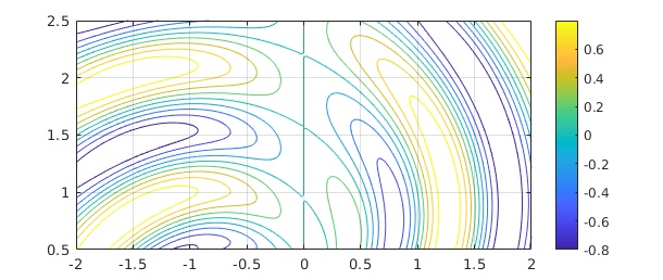
Using 1D Chebfun technology, we can compute the integral over the box like this.
  Iy = @(y) sum(chebfun(@(x) f(x,y),[-2 2]));
  tic, I = sum(chebfun(@(y) Iy(y),[0.5 2.5])); t = toc;
  fprintf('CHEBFUN:  I = %16.14f  time = %5.3f secs\n',I,t)
CHEBFUN: I = 0.02041246545700 time = 0.223 secs
Here for comparison is MATLAB's integral2 with a tolerance of $10^{-11}$:
  tic, I = integral2(f,-2,2,0.5,2.5,'abstol',1e-11,'reltol',1e-11); t = toc;
  fprintf(' MATLAB:  I = %16.14f  time = %5.3f secs\n',I,t)
MATLAB: I = 0.02041246545689 time = 0.068 secs
This example of a 2D integrand is smooth, so both Chebfun and integral2 can handle it to high accuracy.
A much better approach for this problem, however, is to use Chebfun2, which is described in Chapters 12-15. With this method we can compute the integral quickly,
tic
f2 = chebfun2(f,[-2 2 0.5 2.5]);
sum2(f2)
toc
ans =
   0.020412465456998
Elapsed time is 0.197406 seconds.
and we can plot the function without the need for meshgrid:
contour(f2,-1:.2:1), colorbar, grid on

2.6 Gauss and Gauss-Jacobi quadrature
For quadrature experts, Chebfun contains some powerful capabilities due to Nick Hale and Alex Townsend [Hale & Townsend 2013] and Ignace Bogaert [Bogaert, Michiels & Fostier 2012, Bogaert 2014]. To start with, suppose we wish to carry out $4$-point Gauss quadrature over $[-1,1]$. The quadrature nodes are the zeros of the degree $4$ Legendre polynomial legpoly(4), which can be obtained from the Chebfun command legpts, and if two output arguments are requested, legpts provides weights also:
[s,w] = legpts(4)
s =
  -0.861136311594053
  -0.339981043584856
   0.339981043584856
   0.861136311594053
w =
  Columns 1 through 3
   0.347854845137454   0.652145154862546   0.652145154862546
  Column 4
   0.347854845137454
To compute the $4$-point Gauss quadrature approximation to the integral of $\exp(x)$ from $-1$ to $1$, for example, we could now do this:
  x = chebfun('x');
  f = exp(x);
  Igauss = w*f(s)
  Iexact = exp(1) - exp(-1)
Igauss =
   2.350402092156377
Iexact =
   2.350402387287603
There is no need to stop at $4$ points, however. Here we use $1000$ Gauss quadrature points:
  tic
  [s,w] = legpts(1000); Igauss = w*f(s)
  toc
Igauss =
   2.350402387287602
Elapsed time is 0.013837 seconds.
Even a million points doesn't take very long:
  tic
  [s,w] = legpts(1e6); Igauss = w*f(s)
  toc
Igauss =
   2.350402387287601
Elapsed time is 0.084822 seconds.
Traditionally, numerical analysts computed Gauss quadrature nodes and weights by the eigenvalue algorithm of Golub and Welsch [Golub & Welsch 1969]. However, the Hale-Townsend and Bogaert algorithms are both more accurate and much faster [Hale & Townsend 2013, Bogaert, Michiels & Fostier 2012, Bogaert 2014].
For Legendre polynomials, Legendre points, and Gauss quadrature, use legpoly and legpts. For Chebyshev polynomials, Chebyshev points, and Clenshaw-Curtis quadrature, use chebpoly and chebpts and the built-in Chebfun commands such as sum. A third variant is also available: for Jacobi polynomials, Gauss-Jacobi points, and Gauss-Jacobi quadrature, see jacpoly and jacpts. These arise in integration of functions with singularities at one or both endpoints, and are used internally by Chebfun for integration of chebfuns with singularities (Chapter 9). See also hermpts and lagpts.
As explained in the help texts, all of these operators work on general intervals $[a,b]$, not just on $[-1,1]$.
2.7 References
[Assheton 2008] P. Assheton, Comparing Chebfun to Adaptive Quadrature Software, dissertation, MSc in Mathematical Modelling and Scientific Computing, Oxford University, 2008.
[Bogaert 2014] I. Bogaert, "Iteration-free computation of Gauss-Legendre quadrature nodes and weights", SIAM Journal on Scientific Computing, 36 (2014), A1008--A1026.
[Bogaert, Michiels, & Fostier 2012] I. Bogaert, B. Michiels, and J. Fostier, "O(1) computation of Legendre polynomials and Legendre nodes and weights for parallel computing", SIAM Journal on Scientific Computing, 34 (2012), C83-C101.
[Espelid 2003] T. O. Espelid, "Doubly adaptive quadrature routines based on Newton-Cotes rules", BIT Numerical Mathematics, 43 (2003), 319-337.
[Gentleman 1972] W. M. Gentleman, "Implementing Clenshaw-Curtis quadrature I and II", Journal of the ACM, 15 (1972), 337-346 and 353.
[Golub & Welsch 1969] G. H. Golub and J. H. Welsch, "Calculation of Gauss quadrature rules", Mathematics of Computation, 23 (1969), 221-230.
[Gonnet 2009] P. Gonnet, Adaptive Quadrature Re-Revisited, ETH dissertation no. 18347, Swiss Federal Institute of Technology, 2009.
[Hale & Townsend 2013] N. Hale and A. Townsend, Fast and accurate computation of Gauss-Legendre and Gauss-Jacobi quadrature nodes and weights, SIAM Journal on Scientific Computing, 35 (2013), A652-A674.
[Hale & Trefethen 2012] N. Hale and L. N. Trefethen, Chebfun and numerical quadrature, Science in China, 55 (2012), 1749-1760.
[Kahaner 1971] D. K. Kahaner, "Comparison of numerical quadrature formulas", in J. R. Rice, ed., Mathematical Software, Academic Press, 1971, 229-259.
[Kotnik 2008] T. Kotnik, "The prime-counting function and its analytic approximations", Advances in Computational Mathematics, 29 (2008), 55-70.
[Wolfram 2003] S. Wolfram, The Mathematica Book, 5th ed., Wolfram Media, 2003.