1.1 What is a chebfun?
A chebfun is a function of one variable defined on an interval $[a,b]$. The syntax for chebfuns is almost exactly the same as the usual MATLAB syntax for vectors, with the familiar MATLAB commands for vectors overloaded in natural ways. Thus, for example, whereas sum(f) returns the sum of the entries when f is a vector, it returns a definite integral when f is a chebfun.
Chebfun with a capital C is the name of the software system.
The aim of Chebfun is to "feel symbolic but run at the speed of numerics". More precisely, our vision is to achieve for functions what floating-point arithmetic achieves for numbers: rapid computation in which each successive operation is carried out exactly apart from a rounding error that is very small in relative terms [Trefethen 2007].
The implementation of Chebfun is based on the mathematical fact that smooth functions can be represented very efficiently by polynomial interpolation in Chebyshev points, or equivalently, thanks to the Fast Fourier Transform, by expansions in Chebyshev polynomials. For a simple function, 20 or 30 points often suffice, but the process is stable and effective even for functions complicated enough to require 1000 or 1,000,000 points. Chebfun makes use of adaptive procedures that aim to find the right number of points automatically so as to represent each function to roughly machine precision, that is, about 15 or 16 digits of relative accuracy. (Originally Chebfun stored function values at Chebyshev points; in Version 5 it switched to storing Chebyshev expansion coefficients.)
The mathematical foundations of Chebfun are for the most part well established by results scattered throughout the 20th century. A key early figure, for example, was Bernstein in the 1910s. Much of the relevant material can be found collected in the Chebfun-based book Approximation Theory and Approximation Practice [Trefethen 2013].
Chebfun was originally created by Zachary Battles and Nick Trefethen at Oxford during 2002-2005 [Battles & Trefethen 2004]. Battles left the project in 2005, and soon four new members were added to the team: Ricardo Pachon (from 2006), Rodrigo Platte (from 2007), and Toby Driscoll and Nick Hale (from 2008). In 2009, Asgeir Birkisson and Mark Richardson also became involved, and other contributors included Pedro Gonnet, Joris Van Deun, and Georges Klein. Nick Hale served as Director of the project during 2010-2014. The Chebfun Version 5 rewrite was directed by Nick Hale during 2013-2014, and the team included Anthony Austin, Asgeir Birkisson, Toby Driscoll, Hrothgar, Mohsin Javed, Hadrien Montanelli, Alex Townsend, Nick Trefethen, Grady Wright, and Kuan Xu. October 2014 brough new arrivals Jared Aurentz, and Behnam Hashemi. In 2019 the team includes also Nicolas Boulle, Abi Gopal, Yuji Nakatsukasa, and Ryan Sherbo. Further information about Chebfun history is available at the Chebfun web site, http://www.chebfun.org, where one can also find a discussion of other software projects related to Chebfun. This Guide is based on Chebfun Version 5.7.0, released in June 2017.
1.2 Constructing simple chebfuns
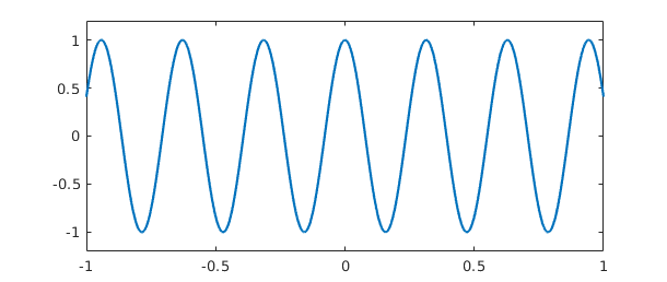
The chebfun command constructs a chebfun from a specification such as a string or an anonymous function. If you don't specify an interval, then the default interval $[-1,1]$ is used. For example, the following command makes a chebfun corresponding to $\cos(20x)$ on $[-1,1]$ and plots it.
  f = chebfun('cos(20*x)');
  plot(f), ylim([-1.2,1.2])
From this little experiment, you cannot see that f is represented by a polynomial. One way to see this is to find the length of f:
length(f)
ans =
    51
Another is to remove the semicolon that suppresses output:
f
f =
   chebfun column (1 smooth piece)
       interval       length     endpoint values
[      -1,       1]       51      0.41     0.41
vertical scale =   1
These results tell us that f is represented by a polynomial interpolant through 51 Chebyshev points, i.e., a polynomial of degree 50. These numbers have been determined by an adaptive process. We can see the data points by plotting f with the '.-' option:
plot(f,'.-'), ylim([-1.2 1.2])
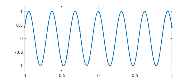
The formula for $N+1$ Chebyshev points in $[-1,1]$ is $$ x(j) = -\cos(j \pi/N), \quad j = 0:N, $$ and in the figure we can see that the points are clustered accordingly near $1$ and $-1$. Note that in the middle of the grid, there are about 5 points per wavelength, which is evidently what it takes to represent this cosine to 15 digits of accuracy. For intervals other than $[-1,1]$, appropriate Chebyshev points are obtained by a linear scaling.
The curve between the data points is the polynomial interpolant, which can be evaluated by the barycentric formula introduced by Salzer [Berrut & Trefethen 2004, Salzer 1972]. This method of evaluating polynomial interpolants is stable and efficient even if the degree is in the millions [Higham 2004]. Chebfun actually evaluates polynomials from their Chebyshev series rather than by barycentric interpolation; the difference in the two methods is little.
What is the integral of $f$ from $-1$ to $1$? Here it is:
sum(f)
ans =
   0.091294525072763
This number was computed by integrating the polynomial (Clenshaw-Curtis quadrature -- see Section 2.1), and it is interesting to compare it to the exact answer from calculus:
exact = sin(20)/10
exact =
   0.091294525072763
Here is another example, now with the chebfun defined by an anonymous function instead of a string. In this case the interval is specified as $[0,100]$.
  g = chebfun(@(t) besselj(0,t),[0,100]);
  plot(g), ylim([-.5 1])
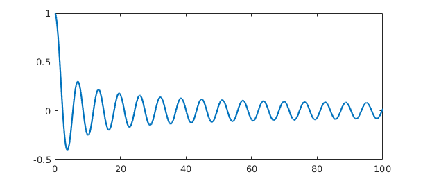
The function looks complicated, but it is actually a polynomial of surprisingly small degree:
length(g)
ans =
    89
Is it accurate? Well, here are three random points in $[0,100]$:
  format long
  x = 100*rand(3,1)
x =
  81.472368639317892
  90.579193707561927
  12.698681629350606
Let's compare the chebfun to the true Bessel function at these points:
  exact = besselj(0,x);
  error = g(x) - exact;
  [g(x) exact error]
ans =
   0.048059538377880   0.048059538377880   0.000000000000000
  -0.021311086924089  -0.021311086924090   0.000000000000000
   0.176415464952875   0.176415464952875  -0.000000000000000
If you want to know the first 5 zeros of the Bessel function, here they are:
r = roots(g); r = r(1:5)
r =
   2.404825557695756
   5.520078110286287
   8.653727912911013
  11.791534439014278
  14.930917708487790
Notice that we have just done something nontrivial and potentially useful. How else would you find zeros of the Bessel function so readily? As always with numerical computation, we cannot expect the answers to be exactly correct, but they will usually be very close. In fact, these computed zeros are accurate to close to machine precision:
besselj(0,r)
ans =
   1.0e-14 *
   0.891222737425086
  -0.809539285445395
   0.010653221425832
  -0.058908346770306
  -0.092296985262750
Most often we get a chebfun by operating on other chebfuns. For example, here is a sequence that uses plus, times, divide, and power operations on an initial chebfun x to produce a famous function of Runge:
  x = chebfun('x');
  f = 1/(1+25*x^2);
  length(f)
  clf, plot(f)
ans =
   187
1.3 Operations on chebfuns
There are more than 300 commands that can be applied to a chebfun. For a list of many of them you can type methods:
methods chebfun
Methods for class chebfun:

abs              csc              jaccoeffs        range
acos             cscd             join             rank
acosd            csch             jump             rdivide
acosh            ctranspose       kron             real
acot             cummax           ldivide          reallog
acotd            cummin           le               realpow
acoth            cumprod          legcoeffs        realsqrt
acsc             cumsum           length           rem
acscd            cylinder         log              remez
acsch            deriv            log10            removeDeltas
airy             diff             log1p            repmat
all              dirac            log2             residue
and              disp             logical          restrict
angle            display          loglog           roots
any              domain           lt               round
arcLength        eigs             lu               sec
area             ellipj           mat2cell         secd
arrowplot        ellipke          max              sech
asec             end              mean             semilogx
asecd            eq               measure          semilogy
asech            erf              merge            sign
asin             erfc             mesh             simplify
asind            erfcinv          min              sin
asinh            erfcx            minandmax        sinc
atan             erfinv           minus            sind
atan2            exp              mldivide         sinh
atan2d           expm             mod              size
atand            expm1            movie            sound
atanh            feval            mpower           spy
besselh          fill             mrdivide         sqrt
besseli          find             mtimes           std
besselj          fix              nchoosek         subsasgn
besselk          fliplr           ne               subspace
bessely          flipud           newDomain        subsref
bvp4c            floor            nextpow2         sum
bvp5c            fracDiff         norm             surf
cat              fracInt          normal           surface
ceil             fred             normest          surfc
cf               gamma            not              svd
cheb2cell        ge               null             tan
cheb2quasi       get              num2cell         tand
chebcoeffs       gmres            or               tanh
chebellipseplot  gt               orth             times
chebfun          heaviside        overlap          transpose
chebpade         horzcat          pde15s           trigcoeffs
chebpoly         hscale           pde23t           trigpade
chebtune         hypot            permute          trigremez
circconv         imag             pinv             truncate
comet            innerProduct     plot             uminus
comet3           integral         plot3            unwrap
complex          inv              plotcoeffs       uplus
compose          isPeriodicTech   plotregion       vander
cond             isdelta          plus             var
conj             isempty          poly             vertcat
conv             isequal          polyfit          volt
cos              isfinite         polyval          vscale
cosd             ishappy          pow2             waterfall
cosh             isinf            power            why
cot              isnan            prod             xor
cotd             isreal           qr
coth             issing           quantumstates
cov              iszero           quasi2cheb

Static methods:

dct              idst             nufft            pchip
dlt              interp1          nufft2           spline
dst              inufft           ode113           update
idct             lagrange         ode15s
idlt             ndct             ode45
To find out what a command does, you can use help.
help chebfun/sum
 SUM   Definite integral of a CHEBFUN.
    SUM(F) is the integral of a column CHEBFUN F over its domain of definition.

    SUM(F, A, B), where A and B are scalars, integrates a column CHEBFUN F over
    [A, B], which must be a subdomain of F.domain:

                          B
                          /
                SUM(F) =  | F(t) dt.
                          /
                         A

    SUM(F, A, B), where A and B are CHEBFUN objects, returns a CHEBFUN S which
    satisfies

                        B(s)
                        /
                S(s) =  | F(t) dt.
                        /
                      A(s)

    SUM(F, DIM), where DIM is one of 1, 2, sums F over the dimension DIM. If F
    is a column CHEBFUN and DIM = 1 or if F is a row CHEBFUN and DIM = 2 then
    this integrates in the continuous dimension of F, as described above.
    Otherwise, SUM(F, DIM) sums across the columns (rows) of the column (row)
    CHEBFUN F.

  See also CUMSUM, DIFF.
Most of the commands in the list above exist in ordinary MATLAB; some exceptions are domain, restrict, and chebcoeffs. We have already seen length and sum in action. In fact we have already seen subsref too, since that is the MATLAB command for (among other things) evaluating arguments in parentheses. Here is another example of its use:
f(0.5)
ans =
   0.137931034482759
Here for comparison is the true result:
1/(1+25/4)
ans =
   0.137931034482759
In this Runge function example, we have also implicitly seen times, plus, power, and rdivide, all of which have been overloaded from their usual MATLAB uses to apply to chebfuns.
In the next part of this tour we shall explore many of these commands systematically. First, however, we should see that chebfuns are not restricted to smooth functions.
1.4 Piecewise smooth chebfuns
Many functions of interest are not smooth but piecewise smooth. In this case a chebfun may consist of a concatenation of smooth pieces, each with its own polynomial representation. Each of the smooth pieces is called a "fun". This enhancement of Chebfun was developed initially by Ricardo Pachon during 2006-2007, then also by Rodrigo Platte starting in 2007 [Pachon, Platte and Trefethen 2010]. Essentially funs are the "classic chebfuns" for smooth functions on $[-1,1]$ originally implemented by Zachary Battles in Chebfun Version 1.
Later we shall describe the options in greater detail, but for the moment let us see some examples. One way to get a piecewise smooth function is directly from the Chebfun constructor, taking advantage of its capability of automatic edge detection. For example, in the default "splitting off" mode a function with a jump in its derivative produces a warning message,
f = chebfun('abs(x-.3)');
Warning: Function not resolved using 65537 pts. Have you tried 'splitting on'?
The same function can be successfully captured with splitting on:
f = chebfun('abs(x-.3)','splitting','on');
The length command reveals that f is defined by four data points, two for each linear interval:
length(f)
ans =
     4
We can see the structure of f in more detail by typing f without a semicolon:
f
f =
   chebfun column (2 smooth pieces)
       interval       length     endpoint values
[      -1,     0.3]        2       1.3        0
[     0.3,       1]        2   5.6e-17      0.7
vertical scale = 1.3    Total length = 4
This output confirms that f consists of two funs, each defined by two points and two corresponding function values. The functions live on intervals defined by breakpoints at $-1$, $1$, and a number very close to $0.3$.
Another way to make a piecewise smooth chebfun is to construct it explicitly from various pieces. For example, the following command specifies three functions $x^2$, $1$, and $4-x$, together with a vector of endpoints indicating that the first function applies on $[-1,1]$, the second on $[1,2]$, and the third on $[2,4]$:
  f = chebfun({@(x) x^2, 1, @(x) 4-x},[-1 1 2 4]);
  plot(f)
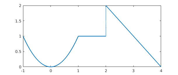
We expect f to consist of three pieces of lengths 3, 1, and 2, and this is indeed the case:
f
f =
   chebfun column (3 smooth pieces)
       interval       length     endpoint values
[      -1,       1]        3         1        1
[       1,       2]        1         1        1
[       2,       4]        2         2        0
vertical scale =   2    Total length = 6
Our eyes see pieces, but to Chebfun, f is just another function. For example, here is its integral.
sum(f)
ans =
   3.666666666666667
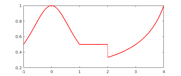
Here is an algebraic transformation of f, which we plot in another color for variety.
plot(1/(1+f),'r')
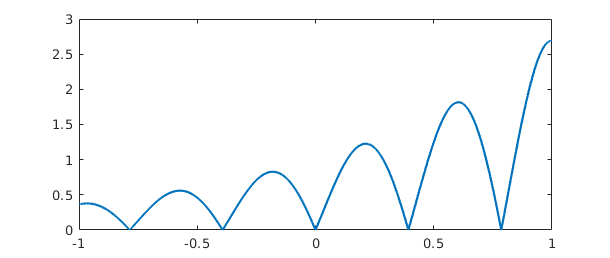
Some Chebfun commands naturally introduce breakpoints in a chebfun. For example, the abs command first finds zeros of a function and introduces breakpoints there. Here is a chebfun consisting of 6 funs:
  f = abs(exp(x).*sin(8*x));
  plot(f)
And here is an example where breakpoints are introduced by the max command, leading to a chebfun with 13 pieces:
  f = sin(20*x);
  g = exp(x-1);
  h = max(f,g);
  plot(h), ylim([0 1.2])
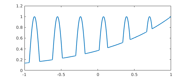
As always, h may look complicated to a human, but to Chebfun it is just a function. Here are its mean, standard deviation, minimum, and maximum:
mean(h)
ans =
   0.578242020778010
std(h)
ans =
   0.280937455806246
min(h)
ans =
   0.135335283236613
max(h)
ans =
   1.000000000000000
A final note about piecewise smooth chebfuns is that the automatic edge detection or "splitting" feature, when it is turned on, may subdivide functions even though they do not have clean point singularities, and this may be desirable or undesirable depending on the application. For example, considering $\sin(x)$ over $[0,1000\pi]$ with splitting on, we end up with a chebfun with many pieces:
tic, f = chebfun('sin(x)',[0 1000*pi],'splitting','on'), toc
f =
   chebfun column (32 smooth pieces)
       interval       length     endpoint values
[       0,      98]       91   2.3e-14    -0.71
[      98,   2e+02]       88     -0.71        1
[   2e+02, 2.9e+02]       88         1    -0.71
[ 2.9e+02, 3.9e+02]       87     -0.71  1.5e-13
[ 3.9e+02, 4.9e+02]       87   2.5e-13     0.71
[ 4.9e+02, 5.9e+02]       87      0.71       -1
[ 5.9e+02, 6.9e+02]       86        -1     0.71
[ 6.9e+02, 7.9e+02]       85      0.71   -6e-13
[ 7.9e+02, 8.8e+02]       86  -9.8e-13    -0.71
[ 8.8e+02, 9.8e+02]       86     -0.71        1
[ 9.8e+02, 1.1e+03]       86         1    -0.71
[ 1.1e+03, 1.2e+03]       86     -0.71 -8.4e-14
[ 1.2e+03, 1.3e+03]       85  -4.3e-13     0.71
[ 1.3e+03, 1.4e+03]       86      0.71       -1
[ 1.4e+03, 1.5e+03]       86        -1     0.71
[ 1.5e+03, 1.6e+03]       85      0.71 -1.3e-12
[ 1.6e+03, 1.7e+03]       86  -9.9e-13    -0.71
[ 1.7e+03, 1.8e+03]       86     -0.71        1
[ 1.8e+03, 1.9e+03]       86         1    -0.71
[ 1.9e+03,   2e+03]       85     -0.71  6.7e-13
[   2e+03, 2.1e+03]       85   1.7e-12     0.71
[ 2.1e+03, 2.2e+03]       86      0.71       -1
[ 2.2e+03, 2.3e+03]       86        -1     0.71
[ 2.3e+03, 2.4e+03]       87      0.71 -1.5e-12
[ 2.4e+03, 2.5e+03]       85     1e-12    -0.71
[ 2.5e+03, 2.6e+03]       86     -0.71        1
[ 2.6e+03, 2.7e+03]       84         1    -0.71
[ 2.7e+03, 2.7e+03]       85     -0.71   -2e-12
[ 2.7e+03, 2.8e+03]       85  -1.2e-14     0.71
[ 2.8e+03, 2.9e+03]       84      0.71       -1
[ 2.9e+03,   3e+03]       86        -1     0.71
[   3e+03, 3.1e+03]       85      0.71 -2.8e-12
vertical scale =   1    Total length = 2752
Elapsed time is 0.265972 seconds.
In this case it is more efficient -- and more interesting mathematically -- to omit the splitting and construct one global chebfun:
tic, f2 = chebfun('sin(x)',[0 1000*pi]), toc
f2 =
   chebfun column (1 smooth piece)
       interval       length     endpoint values
[       0, 3.1e+03]     1684   1.1e-14 -2.8e-13
vertical scale =   1
Elapsed time is 0.035212 seconds.
Splitting on and off are discussed further in Section 8.3.
1.5 Infinite intervals and infinite function values
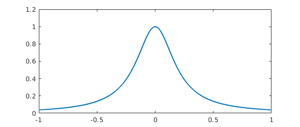
A major change from Chebfun Version 2 to Version 3 was the generalization of chebfuns to allow certain functions on infinite intervals or which diverge to infinity; the initial credit for these innovations belongs to Nick Hale, Rodrigo Platte, and Mark Richardson, and many later developments are due to Kuan Xu. For example, here is a function on the whole real axis,
  f = chebfun('exp(-x^2/16).*(1+.2*cos(10*x))',[-inf,inf]);
  plot(f)
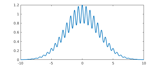
and here is its integral:
sum(f)
Warning: Result may not be accurate as the function decays slowly at infinity.
ans =
   7.089815403622063
Here's the integral of a function on $[1,\infty)$:
sum(chebfun('1/x^4',[1 inf]))
ans =
   0.333333333328451
Notice that several digits of accuracy have been lost here. Be careful! -- operations involving infinities in Chebfun are not always as accurate and robust as their finite counterparts.
Here is an example of a function that diverges to infinity, which we can capture with the 'exps' flag; see Chapter 7 for details:
  h = chebfun('(1/pi)/sqrt(1-x^2)','exps',[-.5 -.5]);
  plot(h)
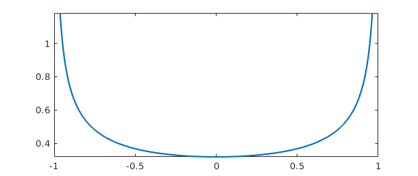
In this case the integral comes out just right:
sum(h)
ans =
   1.000000000000000
For more on the treatment of infinities in Chebfun, see Chapter 9.
1.6 Periodic functions
Until 2014, Chebfun used only nonperiodic representations, based on Chebyshev polynomials. Beginning with Version 5, a new capability was introduced for representing sufficiently smooth periodic functions by trigonometric polynomials instead, that is, Fourier series. Such an object is still called a chebfun, but it is a periodic one, and the signal to invoke such capabilities is the string trig. For abbreviation, we call a periodic chebfun a "trigfun". This section gives a quick introduction, and more details can be found in Chapter 11.
Trigfuns were initiated by Grady Wright in the first half of 2014 [Wright et al. 2015]. Another project along the same lines was carried out independently by Kristyn McLeod and Rodrigo Platte at Arizona State University [McLeod 2014].
For example, here is a periodic function on $[-\pi,\pi]$ represented in the usual way by a Chebyshev series.
ff = @(t) sin(t) + cos(2*t) - cos(t)/3 + cos(100*t)/6;
f = chebfun(ff,[-pi,pi]);
max(f)
plot(f)
ans =
   1.614526099978750
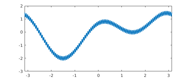
Its length, very roughly, is $100 \pi$,
length(f)
ans =
   383
Here is the same function represented by a Fourier series:
f2 = chebfun(ff,[-pi,pi],'trig');
max(f2)
plot(f2,'m')
ans =
   1.614526099978745
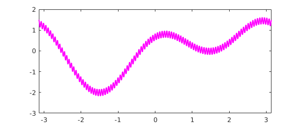
Its length is now only about $200$ (exactly 201). This improvement by a factor of about $\pi/2$ is typical.
length(f2)
ans =
   201
Sampling at a few arbitrary points confirms that the two functions agree closely:
xx = [1/3 sqrt(2) exp(1)];
f(xx) - f2(xx)
ans =
   1.0e-14 *
   0.355271367880050   0.222044604925031   0.111022302462516
Readers may be interested to compare plotcoeffs applied to the first and second versions of $f$. Rather than display that here we shall turn to a simpler example involving a shorter Fourier series. Consider the function
f = chebfun('7 + sin(t) + exp(1)*cos(2*t)',[-pi,pi],'trig')
f =
   chebfun column (1 smooth piece)
       interval       length     endpoint values trig
[    -3.1,     3.1]        5       9.7      9.7
vertical scale = 9.7
Here are the coefficients of $f$ as an expansion in sines and cosines:
[a,b] = trigcoeffs(f)
a =
   7.000000000000000
   0.000000000000001
   2.718281828459045
b =
   1.000000000000000
                   0
Here they are as an expansion in complex exponentials:
c = trigcoeffs(f)
c =
  1.359140914229522 + 0.000000000000000i
  0.000000000000000 + 0.500000000000000i
  7.000000000000000 + 0.000000000000000i
  0.000000000000000 - 0.500000000000000i
  1.359140914229522 + 0.000000000000000i
Bookkeeping of Fourier coefficients can often be a headache. If these examples don't make the patterns clear, details can be found with help trigcoeffs.
For a mathematically less trivial example, here is the cosine expansion of a function whose Fourier series coefficients are known to be values of a Bessel function:
f = chebfun('exp(cos(t))',[-pi pi],'trig');
[a,b] = trigcoeffs(f);
n = floor(length(f)/2);
exact = 2*besseli(0:n,1); exact(1) = exact(1)/2;
disp('        computed             exact')
disp([a exact'])
        computed             exact
   1.266065877752008   1.266065877752008
   1.130318207984970   1.130318207984970
   0.271495339534077   0.271495339534077
   0.044336849848664   0.044336849848664
   0.005474240442094   0.005474240442094
   0.000542926311914   0.000542926311914
   0.000044977322954   0.000044977322954
   0.000003198436462   0.000003198436462
   0.000000199212481   0.000000199212481
   0.000000011036772   0.000000011036772
   0.000000000550590   0.000000000550590
   0.000000000024980   0.000000000024980
   0.000000000001039   0.000000000001039
   0.000000000000040   0.000000000000040
   0.000000000000001   0.000000000000001
1.7 Rows, columns, and quasimatrices
MATLAB doesn't only deal with column vectors: there are also row vectors and matrices. The same is true of Chebfun. The chebfuns shown so far have all been in column orientation, which is the default, but one can also take the transpose, compute inner products, and so on:
x = chebfun(@(x) x)
x =
   chebfun column (1 smooth piece)
       interval       length     endpoint values
[      -1,       1]        2        -1        1
vertical scale =   1
x'
ans =
   chebfun row (1 smooth piece)
       interval       length     endpoint values
[      -1,       1]        2        -1        1
vertical scale =   1
x'*x
ans =
   0.666666666666667
One can also make matrices whose columns are chebfuns or whose rows are chebfuns, like this:
A = [1 x x.^2]
A =
   chebfun column1 (1 smooth piece)
       interval       length     endpoint values
[      -1,       1]        3         1        1
vertical scale =   1
   chebfun column2 (1 smooth piece)
       interval       length     endpoint values
[      -1,       1]        3        -1        1
vertical scale =   1
   chebfun column3 (1 smooth piece)
       interval       length     endpoint values
[      -1,       1]        3         1        1
vertical scale =   1
A'*A
ans =
   2.000000000000000  -0.000000000000000   0.666666666666667
                   0   0.666666666666667   0.000000000000000
   0.666666666666667                   0   0.400000000000000
These are called quasimatrices, and they are discussed in Chapter 6.
1.8 Chebfun features not in this Guide
Some of Chebfun's most remarkable features haven't made it into this edition of the Guide. Here are some of our favorites:
o leg2cheb and cheb2leg for fast Legendre-Chebyshev conversions (also legvals2chebcoeffs, chebcoeffs2legpts, and ten more)
o conv for convolution,
o The 'equi' flag to the Chebfun constructor for equispaced data,
o polyfit for least-squares fitting in the continuous context,
o inv for computing the inverse of a chebfun,
o pde15s for PDEs in one space and one time variable.
To learn about any of these options, try the appropriate help command. Just as a taster, here's a hint of how fast Chebfun can convert a ten-thousand coefficient Chebyshev expansion to Legendre coefficients and back again using an algorithm from [Hale & Townsend 2013]:
tic
ccheb = randn(10000,1);
cleg = cheb2leg(ccheb);
ccheb2 = leg2cheb(cleg);
norm(ccheb-ccheb2,inf)
toc
ans =
     1.905142710256769e-13
Elapsed time is 0.131316 seconds.
1.9 Chebfun example galleries
MATLAB has long had a gallery command to generate interesting matrices, and Chebfun has an analogous gallery command to generate interesting functions.
Here is what is currently available:
help cheb.gallery
CHEB.GALLERY Chebfun example functions.
F = CHEB.GALLERY(NAME) returns a chebfun or a quasimatrix corresponding to
NAME. See the listing below for available names.
For example, plot(cheb.gallery('zigzag')) plots a degree 10000 polynomial
that doesn't look like a polynomial, and plot(cheb.gallery('gamma')) shows
a chebfun with poles. For details of how each function is constructed, try
type +cheb/gallery or edit cheb.gallery.
[F,FA] = CHEB.GALLERY(NAME) also returns the anonymous function FA used to
define the function. Some gallery functions are generated by operations
beyond the usual Chebfun constructor (e.g. by solving ODEs), so FA in those
cases simply evaluates the chebfun.
CHEB.GALLERY with no input argument returns a random function from the
gallery.
CHEB.GALLERY with no output argument creates a plot of the selected
function.
airy Airy Ai function on [-40,40]
bessel Bessel function J_0 on [-100,100]
bump C-infinity function with compact support
blasius Blasius function on [0,10]
chirp Sine with exponentially increasing frequency
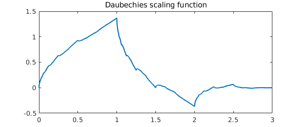
daubechies Approximation to Daubechies phi_2 wavelet scaling function
erf Error function on [-10,10]
fishfillet Wild oscillations from Extreme Extrema example
gamma Gamma function on [-4,4]
gaussian Gaussian function on [-Inf,Inf]
jitter A piecewise constant function generated by ROUND
kahaner Challenging integrand with four spikes
motto Chebfun motto (Gilbert Strang)
random Polynomial interpolant through random data in Chebyshev points
rose A complex-valued sinusoid
runge Runge function
seismograph Tanh plus growing oscillation
Si Sine integral on [-50,50]
sinefun1 As smooth as it looks
sinefun2 Not as smooth as it looks
spikycomb 25 peaks, each sharper than the last
stegosaurus max(wiggly, x/10)
vandercheb Chebyshev-Vandermonde quasimatrix
vandermonde Vandermonde quasimatrix
wiggly One of the Chebfun team's favorites
wild An iteratively defined function on [-1 1]
zigzag Degree 10000 polynomial that looks piecewise linear
Gallery functions are subject to change in future releases of Chebfun.
See also CHEB.GALLERYTRIG, CHEB.GALLERY2, CHEB.GALLERY3, CHEB.GALLERYDISK, CHEB.GALLERYSPHERE.
For example, here is a chebfun representing the Airy function,
plot(cheb.gallery('airy')), ylim([-.8 .8])
title('Airy function')
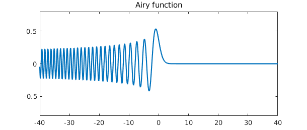
In this instance the underlying code fits in a line,
fa = @airy; p = chebfun(fa, [-40,40]);
Some examples make use of more complicated code, like this approximation to a Daubechies wavelet scaling function (accurate to about 3 digits of accuracy; the underlying function is a fractal):
plot(cheb.gallery('daubechies')), ylim([-0.5 1.5])
title('Daubechies scaling function')
To find out how a gallery example was generated, take a look at the code with type +cheb/gallery or edit +cheb/gallery.
Like the MATLAB gallery command, cheb.gallery produces a plot if you call it without specifying output variables. To illustrate, let us finish with an example the Chebfun team enjoys from the appendix to [Trefethen 2013], "Six myths of polynomial interpolation and quadrature":
cheb.gallery('zigzag')
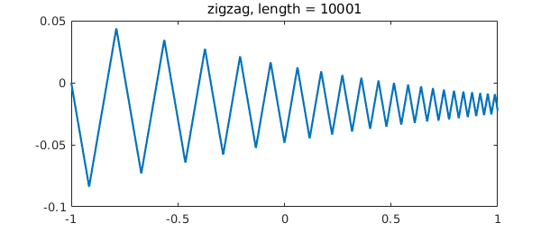
This function looks piecewise linear, but in fact, it is a polynomial of degree 10000. This serves no purpose from an approximation point of view -- one would never represent this function in this manner -- but it illustrates the robustness of high-degree polynomial approximation.
If you call cheb.gallery without any input arguments, it selects a gallery function at random.
Other collections worth exploring include cheb.gallerytrig for periodic functions and cheb.gallery2 for 2D functions.
1.10 How this Guide is produced
This guide is produced in MATLAB using the publish command with a style sheet somewhat different from the usual; the output of publish is then processed by Markdown. To publish a chapter for yourself, make sure the chebfun guide directory is in your path and then type, for example, open(publish('guide1')). The formatting may not be exactly right but it should certainly be intelligible.
1.11 References
[Battles & Trefethen 2004] Z. Battles and L. N. Trefethen, "An extension of MATLAB to continuous functions and operators", SIAM Journal on Scientific Computing, 25 (2004), 1743-1770.
[Berrut & Trefethen 2005] J.-P. Berrut and L. N. Trefethen, "Barycentric Lagrange interpolation", SIAM Review 46, (2004), 501-517.
[Hale & Townsend 2013] N. Hale and A. Townsend, A fast, simple, and stable Chebyshev--Legendre transform using an asymptotic formula, SIAM Journal on Scientific Computing, 36 (2014), A148-A167.
[Higham 2004] N. J. Higham, "The numerical stability of barycentric Lagrange interpolation", IMA Journal of Numerical Analysis, 24 (2004), 547-556.
[McLeod 2014] K. N. McLeod, "Fourfun: A new system for automatic computations using Fourier expansions," SIAM Undergraduate Research Online, 7 (2014), http://dx.doi.org/10.1137/14S013238.
[Pachon, Platte & Trefethen 2010] R. Pachon, R. B. Platte and L. N. Trefethen, "Piecewise-smooth chebfuns", IMA J. Numer. Anal., 30 (2010), 898-916.
[Salzer 1972] H. E. Salzer, "Lagrangian interpolation at the Chebyshev points cos(nu pi/n), nu = 0(1)n; some unnoted advantages", Computer Journal 15 (1972), 156-159.
[Trefethen 2007] L. N. Trefethen, "Computing numerically with functions instead of numbers", Mathematics in Computer Science 1 (2007), 9-19. Revised and reprinted in Communications of the ACM 58 (2014), 91-97.
[Trefethen 2013] L. N. Trefethen, Approximation Theory and Approximation Practice, SIAM, 2013.
[Wright et al. 2015] G. B. Wright, M. Javed, H. Montanelli, and L. N. Trefethen, Extension of Chebfun to periodic functions, SIAM J. Sci. Comp. 37 (2015), C554-C573.