Introduction
The price of a contingent claim can be expressed as the expectation, under the so-called risk-neutral measure, of the payoff discounted to present value. More precisely, consider a contract of European type, which specifies a payoff $V(S_T)$, depending on the level of the underlying asset $S_t$ at maturity $t=T$. The value $V$ of such contract at time $t=0$, conditional to an underlying value $S_0$ is
\begin{equation} V(S_0) = E^Q[e^{-rT} V(S_T)], \label{eq1} \end{equation}
where $E^Q[\cdot]$ denotes the expectation under the risk-neutral measure and $r$ is the risk-free rate.
Such representation of the price is important for theoretical and practical purposes. It suggests a straightforward Monte Carlo based method for its calculation: simulate random paths of the underlying asset; calculate on them the resulting payoff; take the average of the result; discount it by the risk-free rate to present time. This approach is ubiquitous in the financial practice. For an introduction to risk-neutral pricing of financial derivatives, see [1].
In this example we take an alternative route and present a Chebfun-based numerical procedure for the calculation of formula (\ref{eq1}). We have not been able to locate references to a procedure like the one we present here but we wouldn't be surprised if one day we come across them, as it relies on little else than basic probability. (Admittedly, Chebfun makes it look particularly simple.)
Before starting we draw the attention to the related Chebfun example "Black-Scholes PDE using operator exponential" by Toby Driscoll. The object of study in that example is the Black-Scholes PDE, which is connected to the representation of the price in formula (\ref{eq1}) by the Feynman-Kac theorem.
A call option on an asset following a GBM
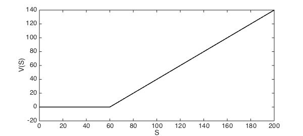
To focus our ideas, we consider the quintessential example of a derivative contract in finance texts: a call option on a stock. It is defined by two parameters, the strike $K$ and the time to expiry $T$, and its payoff is $V(S_T) = \max(0,S_T-K)$.
K = 60;
T = 0.5;
RHSplot = 200;
call = chebfun(@(S) max(0,S-K), [0 K inf]);
LW = 'linewidth';
FS = 'fontsize'; fs = 14;
plot(call,LW,1.6,'k','interval',[0 RHSplot]),
xlabel('S',FS,fs)
ylabel('V(S)',FS,fs);
ylim([-20 140])
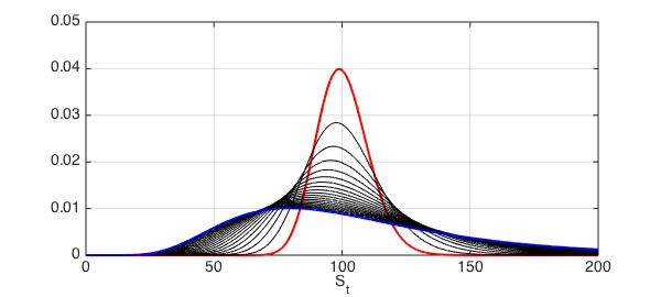
A model for the dynamics of the stock price, with a history stretching back to Sprenkle in 1961 [5], is the geometric Brownian motion. This is a continuous-time stochastic process that specifies at any time $t>0$ a lognormal distribution for the stock price with a probability density function (PDF) $f(S_t)$ of the following form:
$$ f(S_t) = \frac{1}{\sigma S \sqrt{2\pi t}} \exp(\ln(S_t/S_0) - (\mu - \frac12\sigma^2)t)^2/2\sigma^2 t. $$
The parameter $\mu$ is the drift and it determines the trend (e.g., upwards or downwards) that the stock is expected to follow. The parameter $\sigma$ is the volatility, which measures the dispersion of the stock price. The function handle lognHnd below will have these two parameters hard-coded, together with an initial level $S_0$ of the underlying.
mu = 0.075;
vol = 0.45;
S0 = 100;
lognHnd = @(S,t) exp( - ( log(S/S0) - (mu-0.5*vol^2)*t ).^2./(2*vol^2*t) ) ./ ...
    (vol*S*sqrt(2*pi*t));
We wrap the function handle in a chebfun constructor, specifying a right end point large enough for our calculations to be very accurate. The red line shows the PDF at $t=0.05$, the blue line at $t=1$ and the black lines show the PDF at intermediate times, spaced every 0.05 (the unit of time is years).
RHS = 10000;
INT = 'interval';
tvec = 0.05:0.05:1;
for t = tvec
    lognPDF = chebfun(@(S) lognHnd(S,t),[0 RHS]);
    if t == tvec(1), COL ='r'; LWV = 2; elseif t == tvec(end), COL = 'b';
        LWV = 2; else COL = 'k'; LWV = 1; end
    plot(lognPDF,LW,LWV,COL,INT,[0 RHSplot]); hold on,
end
ylim([0 0.05])
xlabel('S_t',FS,fs), set(gca,FS,fs)
set(gca,'YTick',0:0.01:0.05), grid on,
hold off
Our choice for the right end-point should make the area under the curve very close to 1. We check this on the latest lognPDF, which has the heaviest tail to the right:
sum(lognPDF)
ans =
   1.000000000000000
Change from the original to the risk-neutral measure
So far we have only presented the model that the asset price will follow. Now we make the first step for the evaluation of formula (\ref{eq1}), a critical one, which encapsulates the key element of the risk-neutral pricing theory: the probability measure of the process governing the asset has to be changed in such a way that the resulting process is a martingale. The new measure is known as the "risk-neutral measure" and is equivalent (in some sense not discussed here) to the original one.
The possibility of making this change of measure guarantees the lack of arbitrage opportunities in the market (i.e., the possibility of making profit with no risk), an idea found in embryonic form in the seminal work of Black and Scholes [2] and Merton [6], and formalized by Harris and Kreps [3] and Harris and Pliska [4].
For all its conceptual complexity, implementing the change of measure in the case of a GBM process could not be simpler: it consists of replacing the original drift $\mu$ of the stock, with the risk-free rate $r$ of the market. We construct again a function handle lognHnd, but with $r$ instead of $\mu$ and hard-coding the time $t=T$ which is when the call expires.
r = 0.01;
lognHnd = @(S) exp( - ( log(S/S0) - (r-0.5*vol^2)*T ).^2./(2*vol^2*T) ) ./ ...
    (vol*S*sqrt(2*pi*T));
lognPDF = chebfun(@(S) lognHnd(S), [0 RHS]);
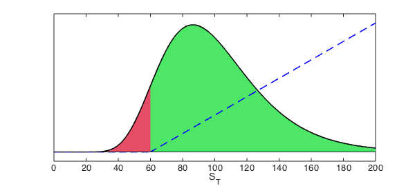
Moneyness
The moneyness of the option refers to the position of the stock price at any point in time before maturity with respect to the strike: if to the left, it is in the "out-of-money" (OOM) region, and if to the right, it is in the "in-the-money" (ITM) region. In our particular setting, if the stock price is, for example, at 50, we would say that the option is OOM, and if it is at 200 we would say that it is deep ITM, highlighting in this way that its is to the right, far from the strike.
The following figure superimposes the terminal PDF of the stock with the payoff profile, both being functions of the stock price at time $T$. Notice that vertical scales of both lines are different, and the Y-axes are omitted to avoid confusion.
OOM_area = area(lognPDF{0,K}); hold on
ITM_area = area(lognPDF{K,RHSplot});
set(OOM_area,'FaceColor',[0.9 0.3 0.4]), axis auto
set(ITM_area,'FaceColor',[0.3 0.9 0.4]), axis auto
plot(lognPDF,INT,[0 RHSplot],LW,1.6,'k'); hold on
set(gca,'YTick',[])
plot(1e-4*call,INT,[0 RHSplot],LW,1.6,'b--');
ylim([-0.001 0.015]), xlabel('S_T',FS,fs)
set(gca,'YTick',[]); hold off
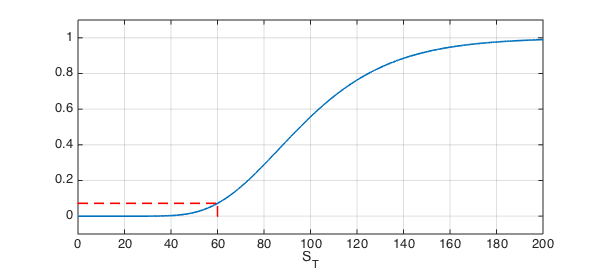
What is the probability that the option expires OOM? To calculate this value, first we use the cumsum command to obtain the cumulative distribution function (CDF) and then we evaluate it in the strike:
lognCDF = cumsum(lognPDF);
probOOM = lognCDF(K)
plot(lognCDF,INT,[0 RHSplot], LW,1.6),
ylim([-.1 1.1]), hold on
plot([K K],[0 probOOM],'r--',LW,1.6),
plot([0 K],[probOOM probOOM], 'r--',LW,1.6)
xlabel('S_T',FS,fs)
hold off, grid on
probOOM =
   0.071872726768390
Distribution of the option payoff at maturity
Formula (\ref{eq1}) takes the risk-neutral expectation of the random variable $V(S_T)$, where $V$ is the function specifying the contract's payoff. How can we calculate the distribution of a random variable which is itself the function of another random variable? The answer of this question appears in every book of basic probability: if $f(x)$ is the PDF of the random variable $x$ and $y(x)$ is a function of $x$, the distribution $g(y)$ is given by
\begin{equation} g(y) = f(x(y))\ \Big|dx/dy\Big|. \label{eq2} \end{equation}
The validity of this rule relies on some assumptions, the most relevant for us now being the possibility of inverting the function $V$, which in turn implies the requirement of the function being monotonically increasing or decreasing. The usual way of dealing with this requirement is to split the domain of the function in regions with this behaviour and then putting them together.
For the case of the call option, we can apply directly this rule on the ITM region to find out its contribution to the PDF of $V(S)$. In this region, the transformation function simply is $y = S-K$ and $dx/dy=1$. Substituting in (\ref{eq2}), we find that the chebfun of the PDF in the ITM region is
ITM = chebfun(@(S) lognHnd(S+K)*1,[0 RHS]);
Notice that the domain of the ITM density function corresponds to the range of $y=S-K$ for $S\geq K$, i.e. $[0,\infty)$. As before, we have used the value RHS to specify the right end-point.
The PDF of constant functions $y(x)=c$ is a Dirac impulse located at $c$ and weight equal to the probability of falling in that region. In the case of the call option, this corresponds to a Dirac delta at zero with weight equal to the probability of ending OOM.
x = chebfun('x',[0 RHS]);
OOM = 2*probOOM*dirac(x);
The domain of the OOM is the point zero, but we constructed its chebfun on the domain [0,RHS] so we can add it with the ITM chebfun. We can obtain now the PDF of $e^{-rT}V(S_T)$ simply as the discounted sum of the two components.
payoffPDF = exp(-r*T)* ( OOM + ITM );
payoffPDF_area = area(payoffPDF{0,RHSplot});
set(payoffPDF_area,'FaceColor',[0.3 0.9 0.4]), axis auto
hold on,
plot(payoffPDF,LW,1.6,'k','deltaline','r'), grid on
xlabel('e^{-rT}V(S_T)',FS,fs)
xlim([-10 RHSplot])
hold off
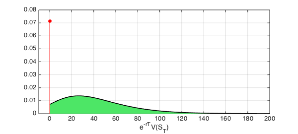
As before, we can check the accuracy by calculating the area under the curve of the undiscounted PDF:
sum(exp(r*T)*payoffPDF)
ans =
   1.000000000001234
Comparison with the Black-Scholes formula
The final step for the pricing of the call option is the calculation of the expected value of the distribution we just obtained:
approx = sum(x.*payoffPDF);
disp(['approx = ', num2str(approx,'%10.15f')])
approx = 40.837802467835829
We indicate the location of the expected value with a blue line on the payoff's distribution.
hold on
plot([approx approx],[0 0.04],'b--',LW,1.6)
hold off
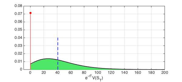
Notice that since the location of the Dirac delta in this example is at zero, the inclusion of the OOM component makes no difference when computing the expected value and we could have skip its construction.
The whole calculation we just did can be done analytically and the result is the celebrated Black-Scholes formula (very similar expressions had been produced before by Sprenke and Samuelson, but without the key insight of changing the measure [5]):
$$ V(S_0) = N(d_1) S - N(d_2) K e^{-rT}, $$
where
$$ d_1 = \frac{1}{\sigma\sqrt{T}} \Bigl( \ln\Bigl(\frac{S}{K}\Bigr) + \Bigl(r+\frac{\sigma^2}{2} \Bigr)T \Bigr), \ \ \ \ d_2 = d_1 - \sigma \sqrt{T}, $$
and $N(\cdot)$ is the CDF of the standard normal distribution. We leave the interpretation of the different elements in this formula to another example, but we can use it now to check the accuracy of our calculation:
d1 = (log(S0./K) + (r+0.5*vol.^2).*T)./(vol.*sqrt(T));
d2 = d1 - vol.*sqrt(T);
exact = S0 .* normcdf(d1) - K .* normcdf(d2) .* exp(-r .* T);
disp(['exact  = ', num2str(exact,'%10.15f')])
disp(['approx = ', num2str(approx,'%10.15f')])
exact  = 40.837802467836617
approx = 40.837802467835829
Summary
In this example we have shown a Chebfun-based method for the pricing of a European call option. The method is conceived in the framework of risk- neutral pricing theory, and by "computing with density functions instead of numbers", we have managed to avoid the Monte Carlo simulation approach.
The easy implementation in Chebfun and the high accuracy obtained are promising features but further experiments need to be done, with different contracts and distributions, to have a better understanding of its pros and cons.
We end this example by listing the steps of the method when applied to a general European derivative (that is, one that is not path-dependent):
-
Construct a chebfun for the PDF/CDF of the underlying asset at maturity under the risk-neutral measure (change $\mu$ for $r$).
-
Split the payoff profile in regions where it is monotonically increasing, monotonically decreasing, or constant. Construct chebfuns for each piece.
-
Calculate the total probability of ending in constant regions and use them as weight of Dirac deltas located at points equal to the constant values. For increasing/decreasing regions, obtain the function $y(x)$ in formula (\ref{eq2}), invert it to obtain $x(y)$ and then differentiate it to obtain $dx/dy$; obtain the composition $f(x(y))$ and calculate the contributions with formula (\ref{eq2}).
-
Add all contributions to obtain the payoff's distribution at maturity.
-
Use the
sumcommand to obtain the expected value of the distribution and discount it by the risk-free rate.
References
-
M. Baxter and A. Rennie, Financial Calculus: An Introduction to Derivative Pricing, CUP, 1996.
-
F. Black and M. Scholes, "The pricing of options and corporate liabilities", Journal of Political Economy 81 (1973), 637--654.
-
M. Harrison and D. M. Kreps, "Martingales and arbitrage in multiperiod securities markets", Journal of Economic Theory 20 (1979), 381--408.
-
M. Harrison and S. Pliska, "Martingales and stochastic integrals in the theory of continuous trading", Stochastic Processes and their Applications 11 (1981), 215--260.
-
D. MacKenzie, An Engine, not a Camera: How Financial Models Shape Markets, MIT Press, 2008.
-
R. C. Merton, "Theory of rational option pricing", Bell Journal of Economics and Management Science 4 (1973), 141--183.