Nearest orthonormal functions

function NearestOrthFun()

Introduction

Suppose $A$ is a given $m \times n$ matrix. The problem of finding the orthonormal matrix $Q$ nearest to $A$ is well-known [4] (by an orthonormal matrix, we mean a matrix with orthonormal columns). Specifically, it is the following problem: $$ Q = \mbox{argmin}_W ||A-W||_\mbox{fro} \quad\mbox{subject to}\quad W^T W = I. $$ This problem is a special case of the orthogonal Procrustes problem [3, p. 327]. There are different ways to find the unique solution to this problem. One way that expresses $Q$ explicitly requires finding a matrix inverse square root [6] as follows:

$$ Q = A(A^T A)^{-1/2}. $$

However, the simplest (and possibly a numerically more stable) way is to compute the singular value decomposition of $A$ and to replace the singular values by ones. In other words, if $A = U S V^T$, then $Q = U V^T$ is the nearest orthonormal matrix to $A$. This is actually the unitary factor in the polar decomposition of $A$ [4].

Our goal is to generalize this situation to the continuous case. Suppose that a set of functions defined on a domain are given. We know how to use Chebfun's qr command to compute orthogonal functions (stored as the columns of a qusimatrix Q2) corresponding to our given functions. See e.g. [2, Ch. 6] for details. Here, we are looking for the nearest set of orthonormal functions. In Chebfun this is also straightforward. We just need to create a quasimatrix out of our given set of functions and use Chebfun's overloaded svd command [1]. The function [Q,Q2] = nearestOrtho(A) in the following computes both Q and Q2.

The first six monomials

A = cheb.gallery('vandermonde'); % A = [1, x, x.^2, x.^3, x.^4, x.^5];
[Q,Q2] = nearestOrtho(A);

Departure from orthogonality in the columns of A = 1.35
Departure from orthogonality in the columns of Q = 2.1e-15
Departure from orthogonality in the columns of Q2 = 1.7e-15
The distance between A and Q2 = 1.92
The distance between A and its closest orthonormal quasimatrix = 1.69

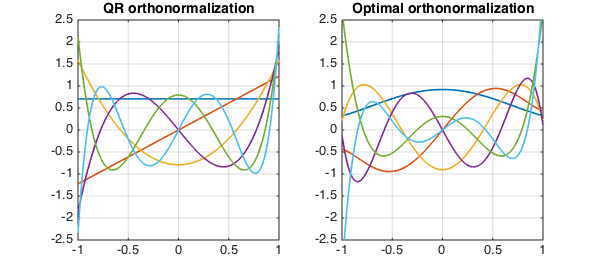
Here, we see Legendre polynomials scaled to have norm 1 (left) and the nearest set of orthonormal functions (right). The first polynomial among these nearest orthonormal polynomials is approximately the following: $ p(x) = 0.9200 - 0.9035 x^2 + 0.3084 x^4$.

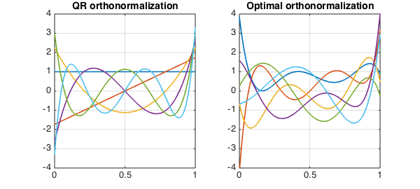
Chebyshev-Vandermonde quasimatrix on the interval [0, 1]

A = cheb.gallery('vandercheb');
A = restrict(A,[0,1]);
[Q,Q2] = nearestOrtho(A);

Departure from orthogonality in the columns of A = 1.00
Departure from orthogonality in the columns of Q = 2.8e-15
Departure from orthogonality in the columns of Q2 = 1.7e-15
The distance between A and Q2 = 2.48
The distance between A and its closest orthonormal quasimatrix = 1.62

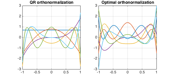
Mixed algebraic and trigonometric example

x = chebfun('x'); A = [1, cos(x), sin(x.^2), x.^3, x.^4, x.^5];
[Q,Q2] = nearestOrtho(A);

Departure from orthogonality in the columns of A = 2.69
Departure from orthogonality in the columns of Q = 5.1e-15
Departure from orthogonality in the columns of Q2 = 5.7e-15
The distance between A and Q2 = 2.43
The distance between A and its closest orthonormal quasimatrix = 1.95

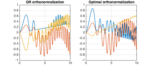
Non-smooth functions on the interval [0,10]

A = [cheb.gallery('stegosaurus'), cheb.gallery('wiggly'), cheb.gallery('blasius')];
[Q,Q2] = nearestOrtho(A);

Departure from orthogonality in the columns of A = 194.38
Departure from orthogonality in the columns of Q = 1.4e-15
Departure from orthogonality in the columns of Q2 = 3.8e-16
The distance between A and Q2 = 13.63
The distance between A and its closest orthonormal quasimatrix = 13.23

A further comment

We mentioned in the introduction that the nearest orthonormal matrix $Q$ to a given matrix $A$ is the orthonormal factor of a polar deomposition $A = QH$. The other factor $H$ is a Hermitian matrix. Analogously, in the case considered in this Example of functions rather than vectors, we are computing the nearest orthognormal quasimatrix $Q$ to a given quasimatrix $A$, and that could be regarded again as half of a polar decomposition $A = QH$. Here both $A$ and $Q$ are quasimatrices, but $H$ is again a fully discrete matrix. The Chebfun team may introduce at a later date a Chebfun command POLDEC to compute the polar decomposition (analogous to Higham's POLDEC command for matrices in the Matrix Computations Toolbox [5]), in which case, this example could be simplified.

function [Q,Q2] = nearestOrtho(A)
[U,S,V] = svd(A);
Q = U*V'; % nearest quasimatrix to A with orthonormal columns

[Q2,R] = qr(A);

m = size(A,2);
figure;
subplot(1,2,1);
plot(Q2);
v=axis; v(4) = -v(3); axis(v); % make the scales look better
grid on; title('QR orthonormalization')
subplot(1,2,2);
plot(Q); axis(v); grid on; title('Optimal orthonormalization')
fprintf(['Departure from orthogonality in the columns' ...
    ' of A = %3.2f\n'], norm(A'*A-eye(m)))
fprintf(['Departure from orthogonality in the columns' ...
    ' of Q = %3.2g\n'], norm(Q'*Q-eye(m)))
fprintf(['Departure from orthogonality in the columns' ...
    ' of Q2 = %3.2g\n'], norm(Q2'*Q2-eye(m)))
fprintf('The distance between A and Q2 = %3.2f\n', norm(A-Q2,'fro'))
fprintf(['The distance between A and its closest orthonormal' ...
    ' quasimatrix = %3.2f\n'], norm(A-Q,'fro'))
end

References

Z. Battles and L.N. Trefethen, An extension of MATLAB to continuous functions and operators, SIAM J. Scientific Computing 25 (2004) 1743-1770.
T.A. Driscoll, N. Hale, and L.N. Trefethen, editors, Chebfun Guide, Pafnuty Publications, Oxford, 2014.
G.H. Golub and C.F. Van Loan, Matrix Computations, 4th edition, The Johns Hopkins University Press, 2013.
N.J. Higham, Matrix nearness problems and applications, pp. 1-27, in Applications of Matrix Theory, Inst. Math. Appl. Conf. Ser. New Ser., Vol. 22, Oxford Univ. Press, New York, 1989.
N.J. Higham, The matrix computation toolbox, http://www.ma.man.ac.uk/~higham/mctoolbox/, 2008.
B.K.P. Horn, H.M. Hilden, and S. Negahdaripour, Closed-form solution of absolute orientation using orthonormal matrices, Journal of the Optical Society A, 5 (1988) 1127-1135.

end