Approximations and oscillation of error

Introduction

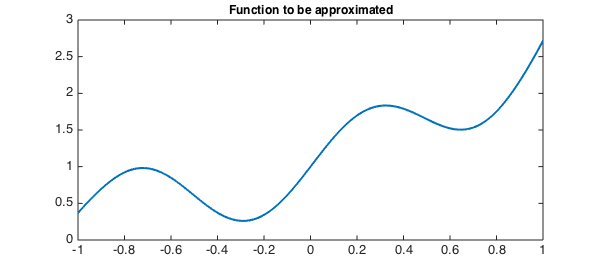
Let us approximate a continuous function $f$ defined on $[-1,1]$ in several different ways.

f = chebfun( @(x) exp(x) + .5*sin(2*pi*x), 10);
LW = 'linewidth'; lw = 2; FS = 'fontsize'; fs = 12;
plot(f, LW, lw),
title( 'Function to be approximated', FS, fs), hold on

Best Approximation in $\infty$-Norm

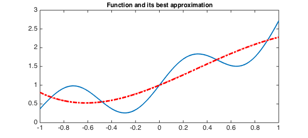
The existence and uniqueness of the the best minimax approximation of $f$ in the space of polynomials of degree up to $n$ is well known. The best degree $n$ approximation is characterized by the equioscillation of the error between at least $n+2$ extrema. The error consequently changes sign at least $n+1$ times [1]. Let us suppose we want to find the degree $n$ best approximation of this function. Chebfun's remez command can be used to find this polynomial:

n = 4;
p = remez(f, n);
plot(p, 'r-.', LW, lw)
title('Function and its best approximation', FS, fs), hold off

clf, hold on
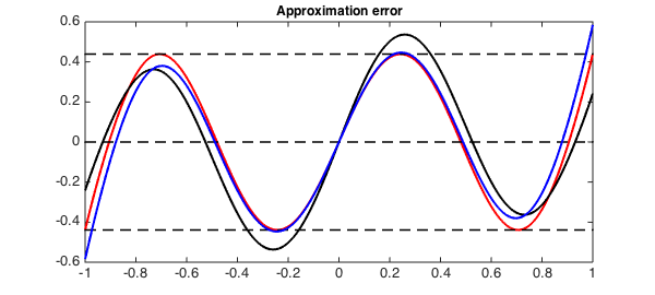
h1 = plot(f - p, 'r', LW, lw);
title('Approximation error', FS, fs)
maxError = norm(f-p, inf);
plot( [-1, 1], [maxError maxError], 'k--', LW, 1.5)
plot( [-1, 1], -[maxError maxError], 'k--', LW, 1.5)
plot( [-1, 1], [0 0], 'k--', LW, 1.5), box on

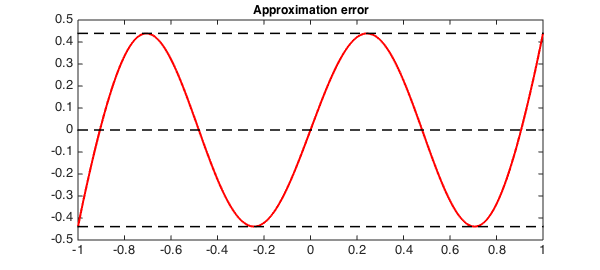
We can see that the error equioscillates $n+2$ times with $n+1$ sign changes.

Best Weighted $L_2$ Approximation

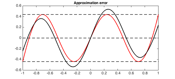
It is also interesting to note that the error curve of the best weighted $L_2$ approximation of a continuous function by a degree $n$ polynomial has the same oscillation property. The error curve is guaranteed to change sign at least $n+1$ times [2], however, in this case, the error curve does not generally equioscillate. For the same function, we now construct a degree $n$ approximation by Chebyshev polynomials. This can be done in Chebfun using the 'trunc' option, since best $L_2$ approximations are simply given by truncated Fourier series (a Chebyshev-Fourier series in this case):

fn = chebfun( @(x) f(x), 'trunc', n + 1);
h2 = plot(f - fn, 'k', LW, lw);

Best $L_2$ Approximation

We can also think of approximating the same function using Legendre polynomials. In this case, we can use Chebfun's polyfit command to generate the best $L_2$ approximating polynomial. This is just the truncated Fourier-Legendre series expansion of the function $f$. The error curve again behaves as expected:

pLn = polyfit(f, n);
h3 = plot(f - pLn, 'b', LW, lw);

Interpolation

The degree $n$ interpolant of a function by definition hits the function normally at least $n+1$ times, and hence the error curve again has at least $n+1$ sign changes.

pn = chebfun( @(x) f(x), n + 1);
h4 = plot( f - pn, 'g', LW, lw); hold off
legend( [h1(:,1), h2(:,1), h3(:,1), h4(:,1)], ...
    {'L_\infty-Best', 'L_2-Cheb', 'L_2-Legn', 'Interp'})

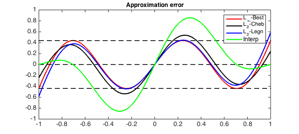
Notice that since Chebfun normally uses Chebyshev points of the second kind for interpolation, which include the end points $-1$ and $1$, the error curve will always have zeros at $-1$ and $1$. You will get a different effect however if you run this example in a mode using Chebyshev points of the first kind rather than the second kind.

References

L. N. Trefethen, Approximation Theory and Approximation Practice, SIAM, 2013.
P. J. Davis, Interpolation and Approximation, Blaisdell Publishing Company, 1965.