LW = 'linewidth'; dom = [0 2*pi];
Chebfun uses Fourier collocation to solve linear, nonlinear and systems of ODEs with periodic boundary conditions. Consider the nonlinear ODE
$$ u' - u\cos(u) = \cos(4x), $$
on $[0, 2\pi]$, with periodic boundary conditions. For nonlinear ODEs, we need to specify an intial guess; let us try $\cos(x)$. We can solve the ODE in Chebfun as follows.
f = chebfun(@(x) cos(4*x), dom);
N = chebop(@(u) diff(u) - u.*cos(u), dom);
N.bc = 'periodic';
N.init = chebfun(@(x) cos(x), dom);
u = N \ f
u =
   chebfun column (1 smooth piece)
       interval       length   endpoint values trig
[       0,     6.3]       89    -0.058   -0.058
Epslevel = 2.331417e-15.  Vscale = 2.428494e-01.
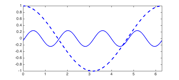
Let us plot the initial guess in dashed blue, and the solution in blue.
figure, plot(N.init, '--b', LW, 2)
hold on, plot(u, 'b', LW, 2)
The solution $u(x)$ satisfies the ODE to high accuracy:
norm(N*u - f, inf)
ans =
     3.379422527647751e-12
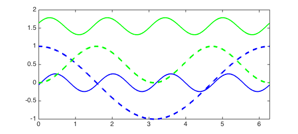
If we start with another initial guess, we might obtain another solution. Let us try $\sin(x)^2$, plot it in dashed green, and plot the solution in green.
N.init = chebfun(@(x) sin(x).^2, dom);
v = N \ f
hold on, plot(N.init, '--g', LW, 2)
hold on, plot(v, 'g', LW, 2)
v =
   chebfun column (1 smooth piece)
       interval       length   endpoint values trig
[       0,     6.3]       81       1.6      1.6
Epslevel = 1.776357e-15.  Vscale = 1.785953e+00.
The solution $v(x)$ satisfies the ODE to high accuracy too:
norm(N*v - f, inf)
ans =
     1.803868478825869e-12
For nonlinear ODEs, the relationships between intial guesses and solutions are difficult to analyse. In this example, we chose two different guesses, and this led to two different solutions.